Discrete two-body reactions

In this section we discuss the calculation of energy depositon to secondary particles for discrete two-body reactions. Suppose that particles 1 and 2 interact to form paricles x and y. Let m_j denote the mass of particle j for j = 1, 2, x, and y, and let v_j be its velocity in the laboratory frame. Then the kinetic of particle j in the laboratory frame is

E_j = $${\frac{{1}}{{2}}}$$m_jv_j²,

We let W_j^* denote the excitation level of the j-th particle, and Q₀ the contribution of the mass difference to the energy of the reaction,

Q₀ = (m₁ + m₂ - m_x - m_y)c². (1)

If particle 2 is at rest in the laboratory frame, then conservation of energy implies that

E₁ + Q = E_x + E_y, (2)

where

Q = Q₀ + (W₁^* + W₂^*) - (W_x^* + W_y^*).

The kinetic energies E_x and E_y of the particles x and y depend on the angles at which they are ejected. The endep code calculates the average values of E_x and E_y based on the probability-density data for the angles ( $\tt I\_number$ = 1 data). Because this data is given in terms of the center-of-mass frame, we have to make a transformation to laboratory coordinates before we compute the average. The arguments given here are based on Newtonian mechanics, so it is assumed that we are dealing with particles that are not too energetic. We shall concentrate our attention on E_x since by a choice of the labels x and y, this represents the kinetic energy of either secondary particle.

The following derivation of a formula for E_x in terms of E₁ and Q is based on the reference [1, pp. 91-94]. The plan of attack is to transform to center-of-mass coordinates and work out the kinematics there, and then transform back to the laboratory frame. We use primes to denote quantities in center-of-mass coordinates. Thus, if V₀ denotes the velocity of the center of mass,

$${\frac{{m_1 v_1 + m_2 v_2}}{{m_1 + m_2}}}$$ (3)

then v₁' = v₁ - V₀, etc. It follows from conservation of momentum that

m₁v₁' = - m₂v₂',

and from this we may derive the relations

$${\frac{{m_2}}{{m_1 + m_2}}} {\frac{{-m_1}}{{m_1 + m_2}}}$$ (4)

These relations are useful because they represent v₁' and v₂' in terms of

v₁' - v₂' = v₁ - v₂ = v₁. (5)

The same momentum conservation argument applied to the secondary particles shows that

$${\frac{{m_y}}{{m_x + m_y}}} {\frac{{-m_x}}{{m_x + m_y}}}$$ (6)

Let us now consider the consequences of energy conservation in the center-of-mass system. It follows from the definition (3) of V₀ that

m₁v₁² + m₂v₂² = (m₁ + m₂)V₀² + m₁v₁'² + m₂v₂'²,

so that E₁ in the the energy equation (2) may be replaced by

E₁ = $${\frac{{1}}{{2}}}$$(m₁ + m₂)V₀² + E₁' + E₂'.

Likewise, under the assumption that m₁ + m₂ $\approx$ m_x + m_y, we may write the right-hand side of (2) as

E_x + E_y = $${\frac{{1}}{{2}}}$$(m_x + m_y)V₀² + E_x' + E_y'.

In writing this equation, we have neglected a term equal to

(m_x + m_y)$$\left(\vphantom{ \frac{m_x v_x + m_y v_y} {m_x + m_y} - V_0 }\right.$$$${\frac{{m_x v_x + m_y v_y}}{{m_x + m_y}}}$$ - V₀$$\left.\vphantom{ \frac{m_x v_x + m_y v_y} {m_x + m_y} - V_0 }\right)$$V₀,

and if this difference is not small relative to Q, we should not be using Newtonian mechanics. In this same vein, upon neglecting the difference

$${\frac{{1}}{{2}}}$$(m_x + m_y - m₁ - m₂)V₀²,

the energy equation in center-of-mass coordinates takes the form

E₁' + E₂' + Q = E_x' + E_y'. (7)

We now perform some algebraic manipulations, using (4) and (6) to derive from (7) an equation for E_x' in terms of E₁. We begin by expressing all of the kinetic energies in terms of squares of velocity differences,

$${\frac{{m_1}}{{2}}} \left(\vphantom{ \frac{m_2} {m_1 + m_2}(v_1' - v_2') }\right. {\frac{{m_2}}{{m_1 + m_2}}} \left.\vphantom{ \frac{m_2} {m_1 + m_2}(v_1' - v_2') }\right)^{2}_{} {\frac{{m_2}}{{2}}} \left(\vphantom{ \frac{m_1} {m_1 + m_2}(v_1' - v_2') }\right. {\frac{{m_1}}{{m_1 + m_2}}} \left.\vphantom{ \frac{m_1} {m_1 + m_2}(v_1' - v_2') }\right)^{2}_{}$$

$${\frac{{m_x}}{{2}}} \left(\vphantom{ \frac{m_y} {m_x + m_y}(v_x' - v_y') }\right. {\frac{{m_y}}{{m_x + m_y}}} \left.\vphantom{ \frac{m_y} {m_x + m_y}(v_x' - v_y') }\right)^{2}_{} {\frac{{m_y}}{{2}}} \left(\vphantom{ \frac{m_x} {m_x + m_y}(v_x' - v_y') }\right. {\frac{{m_x}}{{m_x + m_y}}} \left.\vphantom{ \frac{m_x} {m_x + m_y}(v_x' - v_y') }\right)^{2}_{}$$

Upon combining terms and using the relation (5), we find that

$${\frac{{m_2 E_1}}{{m_1 + m_2}}}$$ + Q = $${\frac{{m_x m_y}}{{2(m_x + m_y)}}}$$(v_x' - v_y')².

If we again use the first of equations (6), we obtain an expression for E_x',

$${\frac{{m_x}}{{2}}} \left(\vphantom{ \frac{m_y} {m_x + m_y} }\right. {\frac{{m_y}}{{m_x + m_y}}} \left.\vphantom{ \frac{m_y} {m_x + m_y} }\right) \left(\vphantom{ \frac{m_2 E_1} {m_1 + m_2} + Q }\right. {\frac{{m_2 E_1}}{{m_1 + m_2}}} \left.\vphantom{ \frac{m_2 E_1} {m_1 + m_2} + Q }\right)$$ (8)

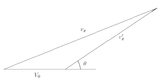
Figure 1: The relationship between velocities.

In order to transform (8) into the laboratory frame, we need a relation between the velocities v_x and v_x' depending on the collision angle $\theta$ in center-of-mass coordinates. In order to do this, we use the fact that v_x is the vector sum of v_x' and the velocity V₀ of the center of mass. See Fig. 1. With the notation that | V₀| is the length of V₀, we find that

v_x² = v_x'² + V₀² +2 | v_x'| | V₀| cos$$\theta$$.

In (8) we make the approximation that m_x + m_y $\approx$ m₁ + m₂. Then, with the notation

$$\alpha {\frac{{m_2 m_y}}{{(m_1 + m_2)^2}}} \beta {\frac{{m_y}}{{m_1 + m_2}}} \gamma {\frac{{m_1 m_x}}{{(m_1 + m_2)^2}}}$$ (9)

it follows from (3) that we have

$$\alpha \gamma \beta \left\{\vphantom{ (\alpha E_1 + \beta Q)\gamma E_1 }\right. \alpha \beta \gamma \left.\vphantom{ (\alpha E_1 + \beta Q)\gamma E_1 }\right\}^{{1/2}}_{} \theta$$ (10)

The library data for the angular distribution ( $\tt I\_number$ = 1 data) is given as the probability density p(E₁,$\eta$) with respect to the center-of-mass collision cosine

$$\eta$$ = cos$$\theta$$.

Consequently, in order to calculate the average secondary energy

$$\langle$$E_x$$\rangle$$ = $$\int_{{-1}}^{1}$$E_xp(E₁,$$\eta$$) d$$\eta$$,

we multiply (10) by p and integrate with respect to $\eta$,

$$\langle \rangle \alpha \gamma \beta \left\{\vphantom{ (\alpha E_1 + \beta Q)\gamma E_1 }\right. \alpha \beta \gamma \left.\vphantom{ (\alpha E_1 + \beta Q)\gamma E_1 }\right\}^{{1/2}}_{} \int_{{-1}}^{1} \eta \eta \eta$$ (11)