Target specific data

This section describes the data in the target specific data section and the ndf access routines used to retrieve this data. To access this data for a specific target one must first call ndfiso to select the target.

Atomic mass: The mass of the target in atomic mass units (AMU). Historically, this was called weight, hence the accessing routines are call ndfatw and ndfcatw for ATomic Weight (atw).

lMax: The maximum Legendre order that data is calculated to and stored in the ndfy_{$\bf i$} file. This is only relevant for the transfer matrix when the incident particle and outgoing particle are the same (i.e., y_i = y_o) and for the transport correcting cross-sections. (When y_i$\ne$ y_o the outgoing particle distribution is assumed to be isotropic; hence, only the l = 0 transfer matrix is stored). See routines ndfmxorder, ndfcmxorder, ndfmxorder_tc and ndfcmxorder_tc.

Total cross-section: The total cross-section is the sum of all the reaction cross-sections described in item Reaction specific information below and has units of barn. The access routines for this data are ndftotal, ndfsig, ndfctotal and ndfcsig.

Transport correcting cross-section: Deterministic transport codes that use a Legendre expansion truncate the expansion due to resource limitations. A truncation at order l_T requires a correction from the next order l_T + 1. This correction is called the transport correcting cross-section in this document and is label tc_l in Table 3 with l = l_T + 1. Four transport correcting cross-section methods are supported by the ndf accessing routines. Table 3 describes the four methods. The default method is Pendlebury/Underhill. Each transport correcting cross-section can be calculated for Legendre order 1 to lMax_tc where lMax_tc is given in column 3 of Table 3. The LLNL exact method has two caveats; (1) the lMax + 1 exact correction is really the LLNL approximate method, (2) if the i^th group total cross-section is less than the exact tc_l(i) then the exact tc_l(i) is replaced by the approximate tc_l(i).

Table 3: List of the four transport correcting algorithm options available through the ndf access routines. TM_l is the l^th Legendre order interaction transfer matrix (see item Transfer matrices), f_l(E) is the l^th Legendre order flux and N₃ is the lesser of i + 3 and ng. lMax_tc is the highest Legendre order available for the specified algorithm.

Code	Name	lMaxtc	tcl(i) (for i = 1 to ng)
0	None	lMax + 1	0
1	Pendlebury/Underhill	lMax	TMl(i, i)
2	LLNL (exact)	lMax	$\sum_{{j=1}}^{{ng}}$fl(j) TMl(i, j)/fl(i)
	LLNL (approximate)	lMax + 1	$\sum_{{j=1}}^{{ng}}$TMl(j, i)
3	Ferguson	lMax	$\sum_{{j=i}}^{{N_3}}$TMl(j, i)

See routines ndfsig, ndftrcorr, ndfcorrec, ndfncorrec, ndfcsig, ndfctrcorr, ndfccorrec and ndfcncorrec. This data has units of barn.

Reaction specific information: Each target contains a list of all reactions included in its processing as well as cross-section and particles produced (including non-transportable particles) for each reaction. A reaction is identified by a unique combination of C, S, Q, X1, X2, X3, and Q _eff-values. The C-value identifies the type of reaction (e.g., C = 10 identifies the reaction as elastic scattering, C = 11 identifies the reaction as inelastic scattering and C = 15 identifies the reaction as fission). Some reaction types are sub-divided as given by the S-, X1-, X2-, and X3-values. As example, for many targets the C = 11, inelastic scattering, reaction is sub-divided into several level excitations (S = 1, X1 = level excitation MeV) and the rest (S = 0). The Q-value is the mass difference of the reaction. Q _eff is the threshold-energy for the reaction, and is typically, but not always, Q _calculated - X1. Q _calculated is calculated during the processing stage from a table of masses, while Q is taken from input data files that may contain slightly different masses; whence Q _eff is close but not always equal to Q - X1. All energy values have units of MeV.

The following two examples illustrate the type of reactions found in a ndfy_{$\bf i$} file. (Note, sometimes there is a difference between the actual particles produced and those found in a ndfy_{$\bf i$} file. During the processing of a ndfy_{$\bf i$} file, the particles produced (i.e., particles occurring on the right hand side of the $\rightarrow$ in Tables 4 and 6) are determined. If a product particle is not in the list of targets in the ndfy_{$\bf i$} file then the processing code substitutes for it a nearby target that is in the ndfy_{$\bf i$} file.) Tables 4 and 5 are an example of a neutron incident on a ⁹Be target. This ndf1 file does not contain the targets ⁹Li, ⁸Li and ⁶He, so they were replaced by the targets ⁷Li, ⁷Li and $\alpha$ respectively. The Q-values are calculated with the actual product particles and not the substituted ones.

Table: Example of the list of reactions for ⁹Be in a ndf1 file. The $\hookrightarrow$ indicates lines that are a duplicate of the line above them except that the product particle substituted by the processing code is listed instead the actual product particle.

n + 9Be $\rightarrow$ n + 9Be	! C = 10, Elastic scattering
n + 9Be $\rightarrow$ n + n + $\alpha$ + $\alpha$	! C = 12, (n,2n)
n + 9Be $\rightarrow$ p + 9Li	! C = 40, (n,p)
$\hookrightarrow$ n + 9Be $\rightarrow$ p + 7Li	! 9Li replaced with 7Li
n + 9Be $\rightarrow$ d + 8Li	! C = 41, (n,d)
$\hookrightarrow$ n + 9Be $\rightarrow$ d + 7Li	! 8Li replaced with 7Li
n + 9Be $\rightarrow$ t + 7Li	! C = 42, (n,t)
n + 9Be $\rightarrow$ $\alpha$ + 6He	! C = 45, (n,$\alpha$)
$\hookrightarrow$ n + 9Be $\rightarrow$ $\alpha$ + $\alpha$	! 6He replaced with $\alpha$
n + 9Be $\rightarrow$ $\gamma$ + 10Be	! C = 46, Capture

Table 5: Actual reaction data for the reactions in Table 4 as stored in a ndf1 file.

C	S	Q	X1	X2	X3	Q eff
10	0	0.	0.	0.	0.	0.
12	0	-1.5728	0.	0.	0.	-1.5728
40	1	-12.83	0.	0.	0.	-12.824
41	1	-14.66	0.	0.	0.	-14.664
42	1	-10.44	0.	0.	0.	-10.439
42	1	-10.44	0.478	0.	0.	-10.917
45	1	-0.6	0.	0.	0.	-0.60175
46	0	6.82	0.	0.	0.	6.82

Tables 6 and 7 are an example of a neutron incident on a ¹⁰B target. Multiple C = 11 entries are present; four with S = 1 for the excitation levels 0.717, 1.74, 2.154 and 3.59 MeV and one with S = 0 for the rest of the inelastic reaction cross-section data.

Table 6: Example of the list of reaction for ¹⁰B in a ndf1 file.

n + 10B $\rightarrow$ n + 10B	! C = 10, Elastic scattering
n + 10B $\rightarrow$ n' + 10B	! C = 11, Inelastic scattering
n + 10B $\rightarrow$ n + d + $\alpha$ + $\alpha$	! C = 23, (n,n d $\alpha$)
n + 10B $\rightarrow$ n + n + p + $\alpha$ + $\alpha$	! C = 31, (n,2n p $\alpha$)
n + 10B $\rightarrow$ t + $\alpha$ + $\alpha$	! C = 43, (n,t $\alpha$)
n + 10B $\rightarrow$ $\alpha$ + 7Li	! C = 45, (n,$\alpha$)
n + 10B $\rightarrow$ $\gamma$ + 11B	! C = 46, Capture

Table 7: Actual reaction data for the reactions in Table 6 as stored in a ndf1 file.

C	S	Q	X1	X2	X3	Q eff
10	0	0.	0.	0.	0.	0.
11	0	0.	0.	0.	0.	0.
11	1	0.	0.717	0.	0.	-0.717
11	1	0.	1.74	0.	0.	-1.74
11	1	0.	2.154	0.	0.	-2.154
11	1	0.	3.59	0.	0.	-3.59
23	0	-6.02	0.	0.	0.	-6.02
31	0	-8.158	0.	0.	0.	-6.02
43	0	0.33	0.	0.	0.	0.33
45	0	2.8	0.	0.	0.	2.8
46	0	11.45	0.	0.	0.	11.45

The access routines allow one to obtain information about the number of reactions, the list of C-values, the summed cross-section and Q-value for a reaction type, and the particles produced for a specific reaction as described below.

Number of reactions: The number of reactions for a specific target is obtained by calling ndfnreact or ndfcnreact. For Tables 5 and 7 the number of reactions are 8 and 11 respectively. Also see routines ndfreact, ndfnrxs, ndfrxs, ndfrxslist, ndfrxslevel, ndfcreact, ndfcnrxs, ndfcrxs, ndfcrxslist and ndfcrxslevel.

Reaction cross-section: Reaction specific, for a specified C-value, cross-section data are obtained by calling ndfrxs or ndfcrxs. Also see routines ndfnrxs, ndfrxslist, ndfrxslevel, ndfcnrxs, ndfcrxslist and ndfcrxslevel. This data has units of barn.

Reaction particles produced: The particles produced for a specified Reaction, C-value, are obtained by calling ndfprod or ndfcprod. As example, for the C = 40 reaction for the data in Table 4, ndfnprod would return 2 and ndfprod would return the lists ZAList = { 2, 3007 } and MList = { 1, 1 } since two particles are produced (i.e., p and ⁷Li), each with multiplicity 1. Also see routines ndfnprod, and ndfcnprod.

Transportable particles produced, (i.e., y_os): Each target produces transportable particles. For example, the ⁹Be target of Table 4 and the ¹⁰B target of Table 6 each produce 6 transportable particles (n, p, d, t, $\alpha$ and $\gamma$). The number of difference transportable particle types produced is obtained by calling ndfnyos or ndfcnyos. A list of transportable particle types produced is obtained by calling ndfyos or ndfcyos. Also see routines ndfnppyos, ndfppyos, ndfcnppyos, and ndfcppyos which are similar but do not include the incident transportable particle in the number of particles produced or the list.

Transfer matrices: The formulas for the transfer matrices will not be presented here; instead, see chapter VI of reference [1] and reference [2]. In summary, three methods can be used to calculate a transfer matrix, depending on whether particle number, energy or number/energy of the outgoing particles is to be conserved during the processing (see item yo descriptor in Section 5.1). Only the particle number conserving transfer matrix is outlined here. The particle number conserving transfer matrix for outgoing particle y_o is defined as,

$$\rightarrow \sum_{{r,{\rm y}_o}}^{} \left(\vphantom{ { \displaystyle \int_{E_{g+1}}^{E_g} \int_{E'_{h... ... \, dE \, dE' \over \displaystyle \int_{E_{g+1}}^{E_g} f^l(E) \, dE } }\right. {\displaystyle \int_{E_{g+1}}^{E_g} \int_{E'_{h+1}}^{E'_h} f^l(E... ...htarrow h} \, dE \, dE' \over \displaystyle \int_{E_{g+1}}^{E_g} f^l(E) \, dE} \left.\vphantom{ { \displaystyle \int_{E_{g+1}}^{E_g} \int_{E'_{h... ... \, dE \, dE' \over \displaystyle \int_{E_{g+1}}^{E_g} f^l(E) \, dE } }\right)$$ (16)

Here, h is the outgoing particle's group designation, $\sum_{{r,{\rm y}_o}}^{}$ means to sum only reactions that produce y_o as an outgoing particle, $\sigma_{r}^{}$(E) and M_{r, yo}(E) are the cross-section and multiplicity respectively for the reaction (e.g., for the C = 13, (n,3n), reaction and yo = 1, M_{13, 1}(E) = 3) and $\pi^{l}_{{r,g \rightarrow h}}$ is the grouped, l^th Legendre coefficient of the normalized probability of the incident particle of energy E producing the required outgoing particle with energy E' at angle $\theta$.

The transfer matrices are divided into two types. The first type is called the interaction transfer matrix and is the transfer matrix when the incident transportable particle type is the same as the outgoing transportable particle type (i.e., y _i $\rightarrow$ y_o for y_i = y_o). The interaction transfer matrix is calculated to Legendre order l = lMax + 1 during processing, so that the lMax + 1 LLNL approximate transport correcting cross-sections can be calculated, but is only stored to order l = lMax in the ndfy_{$\bf i$} file. These matrices are accessed with routines ndfsig, ndftransfer, ndfcsig and ndfctransfer. The second type of transfer matrix is called the production transfer matrix. This matrix is the transfer matrix when the incident transportable particle type is different than the outgoing transportable particle type (i.e., y _i $\rightarrow$ y_o for y_i$\ne$ y_o) and is only calculated for Legendre order l = 0. These matrices are accessed with routines ndfnppyos, ndfppyos, ndfpmat, ndfppmatrix, ndfcnppyos, ndfcppyos, ndfcpmat and ndfcppmatrix. This data has units of barn.

The multiplicity factor in Eq. 16 often leads to confusion with users of the ndf access routines as they assume that the total cross-section must be greater than or equal to the l = 0 interaction transfer matrix integrated over outgoing particle energy; since the sum is only over reactions that produce a specific outgoing particle. To understand the confusion, consider a simple problem with a neutron incident on target X that only has the two reactions C = 10 (n,n) and C = 13 (n,3n). Let both reactions' cross-sections be isotropic, independent of energy and 1 barn. Thus, the l = 0 interaction transfer matrix integrated over outgoing particle energy is 4 barns (1 x 1. barn + 3 x 1. barn) which is greater than the total cross-section of 2 barns.

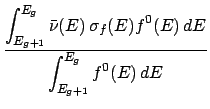
Fission < $\nu$$\sigma_{f}^{}$ > _g: For neutrons produced by fission, C = 15, the multiplicity is dependent on energy and not an integer (since it is an average multiplicity over many possible fission channels). The average number of neutrons produced by fission < $\nu$$\sigma_{f}^{}$ > _g is stored for targets that fission and is calculated as,

$$\nu \sigma_{f}^{} {\displaystyle \int_{E_{g+1}}^{E_g} \bar\nu(E) \, \sigma_f(E) f^0(E) \, dE \over \displaystyle \int_{E_{g+1}}^{E_g} f^0(E) \, dE}$$ (17)

where $\bar{\nu}$(E) is the number of neutrons produced by fission average over possible fission channels and $\sigma_{f}^{}$ is the fission cross-section. This data only occurs for neutron as incident particle (y_i = 1) and when the neutron multiplicity returned by ndfprod or ndfcprod is 0. This data is accessed with routines ndffisx and ndfcfisx, and has units of barn.

Fission neutron transfer matrix: For targets in a ndf1 file that have fission data the l = 0 fission transfer matrix is calculated. It is calculated just like the l = 0 interaction transfer matrix except only the fission reaction data is used. See routines ndffisx ndfifsp, ndffsp, ndfcfisx, ndfcifsp and ndfcfsp. This data has units of barn.

Energy conservation and energy data: To conserve energy, particles that are not transported by a code have to have their energy deposited locally. The amount of energy that must be deposited locally and how to obtain it from a ndfy_{$\bf i$} file is outlined below.

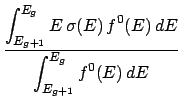
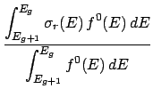
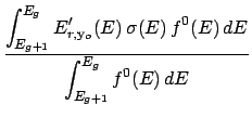
During the processing of a ndfy_{$\bf i$} file, the average kinetic energy of an incident particle in group g is calculated as,

$$\sigma \sum_{r}^{} \left(\vphantom{ { \displaystyle \int_{E_{g+1}}^{E_g} E \, \sigma... ... f^0(E) \, dE \over \displaystyle \int_{E_{g+1}}^{E_g} f^0(E) \, dE } }\right. {\displaystyle \int_{E_{g+1}}^{E_g} E \, \sigma_r(E) \, f^0(E) \, dE \over \displaystyle \int_{E_{g+1}}^{E_g} f^0(E) \, dE} \left.\vphantom{ { \displaystyle \int_{E_{g+1}}^{E_g} E \, \sigma... ... f^0(E) \, dE \over \displaystyle \int_{E_{g+1}}^{E_g} f^0(E) \, dE } }\right) {\displaystyle \int_{E_{g+1}}^{E_g} E \, \sigma(E) \, f^0(E) \, dE \over \displaystyle \int_{E_{g+1}}^{E_g} f^0(E) \, dE}$$ (18)

Here, $\sigma_{r}^{}$(E) is the cross-section for a given reaction and $\sigma$(E) is the total cross-section.

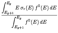
The average energy due to the mass differences between the before and after reaction particles, called the production energy (see item ep below), is calculated as,

$$\sigma \sum_{r}^{} \left(\vphantom{ { \displaystyle \int_{E_{g+1}}^{E_g} \sigma_r(E) \, f^0(E) \, dE \over \displaystyle \int_{E_{g+1}}^{E_g} f^0(E) \, dE } }\right. {\displaystyle \int_{E_{g+1}}^{E_g} \sigma_r(E) \, f^0(E) \, dE \over \displaystyle \int_{E_{g+1}}^{E_g} f^0(E) \, dE} \left.\vphantom{ { \displaystyle \int_{E_{g+1}}^{E_g} \sigma_r(E) \, f^0(E) \, dE \over \displaystyle \int_{E_{g+1}}^{E_g} f^0(E) \, dE } }\right) \sum_{r}^{} \sigma_{{r,g}}^{}$$ (19)

where Q_r is the sum of the incident particle's and target's masses minus the sum of all outgoing particles' masses (this includes non-transportable particles). The sum of Eqs. 18 and 19 is the total available energy (see item emax below),

$$\sigma \sigma \sigma$$ (20)

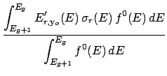
During the processing the average energy deposited to a transportable outgoing particles (see item ed(y_o) below) is calculated as,

$$\sigma \sum_{r}^{} \left(\vphantom{ { \displaystyle \int_{E_{g+1}}^{E_g} E'_{r,{\rm ... ... f^0(E) \, dE \over \displaystyle \int_{E_{g+1}}^{E_g} f^0(E) \, dE } }\right. {\displaystyle \int_{E_{g+1}}^{E_g} E'_{r,{\rm y}_o}(E) \, \sigma_r(E) \, f^0(E) \, dE \over \displaystyle \int_{E_{g+1}}^{E_g} f^0(E) \, dE} \left.\vphantom{ { \displaystyle \int_{E_{g+1}}^{E_g} E'_{r,{\rm ... ... f^0(E) \, dE \over \displaystyle \int_{E_{g+1}}^{E_g} f^0(E) \, dE } }\right) {\displaystyle \int_{E_{g+1}}^{E_g} E'_{r,{\rm y}_o}(E) \, \sigma(E) \, f^0(E) \, dE \over \displaystyle \int_{E_{g+1}}^{E_g} f^0(E) \, dE}$$ (21)

Here E'_{r, yo} is the average energy deposited to a transportable particle of type y_o for reaction r. The amount of energy to be locally deposited is calculated as the total available energy, Eq 20, minus the energy deposited to all transportable outgoing particles that are being transported.

emax: This is the total available energy (Eq. 20) and has units of MeV-barn. This data is accessed using ndfemax or ndfcemax.

ep: This is the production energy (Eq. 19) and has units of MeV-barn. This data is accessed using ndfep or ndfcep.

ed(y_o): This is the average energy deposited to transportable outgoing particle y_o (Eq. 21) and has units of MeV-barn. This data is accessed using ndfsig or ndfcsig when (y_o = y_i) and is accessed using ndfpmat or ndfcpmat when (y_o$\ne$ y_i). Also see routines ndfed, ndfnyos, ndfyos, ndfced, ndfcnyos and ndfcyos.