UCRL-ID-144510

The TDF System for Thermonuclear Plasma Reaction Rates, Mean Energies and Two-Body Final State Particle Spectra

Stephen I. Warshaw

July 11, 2001

N Division
Physics and Advanced Technologies Directorate
Lawrence Livermore National Laboratory
Livermore, CA 94551

Table of Contents

1. Introduction.

2. The Maxwellian-averaged thermonuclear reaction rate

3. Maxwellian-averaged mean energies and cosines for two-body final state reactions

4. Exit particle energies in the t(t,2n)a reaction: a foray into three-body final state energy averaging

5. Maxwellian-averaged two-body final state reaction particle spectra

6. Digression on two-body final state spectrum moments

7. Data, algorithmic bases and results of calculations

8. Algorithmic bases and results for , and

9. Algorithmic basis of the final state spectral probability distributions

10. The Thermonuclear Data File (TDF) generator

11. Structure and content of the TDF

12. The TDFLIB subroutine library

Acknowledgments

Bibliography and References

Appendix A. Example TDF format

Appendix B. Erratum in Williams' original paper

Appendix C. Evaluation of a d function integral over finite limits

1. Introduction

The rate of thermonuclear reactions in hot plasmas as a function of local plasma temperature determines the way in which thermonuclear ignition and burning proceeds in the plasma. The conventional model approach to calculating these rates is to assume that the reacting nuclei in the plasma are in Maxwellian equilibrium at some well-defined plasma temperature, over which the statistical average of the reaction rate quantity sv is calculated, where s is the cross-section for the reaction to proceed at the relative velocity v between the reacting particles. This approach is well-understood and is the basis for much nuclear fusion and astrophysical nuclear reaction rate data. (See, e.g., Chiu 1968, Clayton 1968)

The Thermonuclear Data File (TDF) system developed at the Lawrence Livermore National Laboratory (Warshaw 1991), which is the topic of this report, contains data on the Maxwellian-averaged thermonuclear reaction rates for various light nuclear reactions and the correspondingly Maxwellian-averaged energy spectra of the particles in the final state of those reactions as well. This spectral information closely models the output particle and energy distributions in a burning plasma, and therefore leads to more accurate computational treatments of thermonuclear burn, output particle energy deposition and diagnostics, in various contexts. In this report we review and derive the theoretical basis for calculating Maxwellian-averaged thermonuclear reaction rates, mean particle energies, and output particle spectral energy distributions for these reactions in the TDF system. The treatment of the kinematics is non-relativistic. The current version of the TDF system provides exit particle energy spectrum distributions for two-body final state reactions only. In a future report we will discuss and describe how output particle energy spectra for three- and four-body final states can be developed for the TDF system.

We also include in this report a description of the algorithmic implementation of the TDF system, which is in two parts: the code which generates the data file itself from the nuclear reaction cross-sections, and the lookup utilities (bundled in a Fortran 77 subroutine library) which are used to retrieve the appropriate thermo-nuclear data from the file on demand. Unique approaches to generating, retrieving and looking up the data that were developed will be described in some detail. These developments resulted in an unusually compact data file which can be quickly generated, and from which an enormous amount of thermonuclear reaction rate, output particle energy and particle energy spectrum data can be rapidly retrieved. It is this compactness, speed and relative platform independence that distinguishes the LLNL TDF system from others.

2. The Maxwellian-averaged thermonuclear reaction rate

Consider a plasma containing a mixture of two nuclear species which react to produce other particles and nuclei. We quantify the rate of thermonuclear reaction by first considering a "local" microscopic model in which one of the nuclear species is at rest, and the other is traveling toward the stationary nuclei in a beam moving at velocity v, as shown schematically in Figure 1.

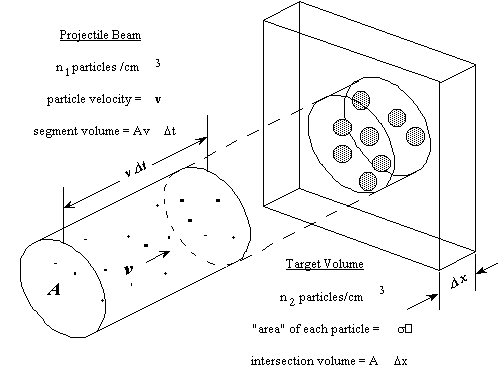
Figure 1. Particle-beam particle-target geometry

With the geometric notions shown in the figure, the number of particles in the beam segment is

where A is the area of the beam cross-section (and therefore the area of the particle interaction volume). The total area presented by the target particles within the particle interaction volume to the particles in the beam is

Thus the fraction of the particle beam that is intercepted by the target particles is

and the total number of beam particle - target particle interactions is therefore

Since the interaction volume is ADx and the interaction time is Dt, we then have that the number of interactions per unit volume per unit time is

This quantity is considered to be the instantaneous local reaction rate density for the binary plasma in question when it is understood that v is the scalar relative velocity

between the nuclei of the different species, the binary interaction cross-section s is strictly a function of v_R, and the particle densities n₁ and n₂ are understood to be locally constant and uniform.

In a plasma the velocities v₁ and v₂ of two interacting component species of particle are distributed in magnitude and direction, so that the number of particles per unit volume of species type 1 having a mean velocity v₁ within the differential cell d³v₁ = dv_1xdv_1ydv_1z in velocity space is

and the number of particles per unit volume of species type 2, similarly, is

where f(v_i) is symbolic for the normalized distribution function for particle species i in the plasma. Then the total reaction rate density for the interacting species in the plasma is the integral of the local reaction rate density over all possible particle pair combinations and vector relative velocities, as follows:

Note that this is an integral over a joint distribution f(v₁)f(v₂). Since the functions f(v_i) are assumed normalized, that is,

this quantity is also the statistical average of n₁n₂sv over the joint distribution, and may therefore be written as

In the case where both reacting particles are identical (as in the d(d,n)³He reaction, for example), the RRD needs to be calculated differently, because during the double integration over dn₁dn₂ the same particle population is integrated over twice. This means that each reacting particle pair is counted twice, and the RRD in this case is double what it should be. The correct formulation of the RRD in the general case is therefore as follows:

where i and j denote the reacting particle species, and d_ij is the Kronecker delta, which is equal to 1 when i = j and 0 otherwise. (This multiplying factor issue is discussed more thoroughly by Clayton (1968)).

Because the particle densities n_i and n_j are particular to a given plasma configuration and so may themselves be distributed in time and space, we have formulated the TDF system to provide only the "bare" statistical average . It therefore does not include the pair count multiplier n_in_j/(1 + d_ij). In this report we treat only the statistical average and ignore the multiplier, as well.

In our modeling we assume the reacting particle species each have an isotropic Maxwellian distribution at a common kinetic temperature q = kT. Then the particle distribution functions for each species also depend on particle mass and plasma temperature, and have the well-known form

where m_i is the particle mass, v_i² is the square of the magnitude of the vector velocity v_i, and i = 1 or 2 identifies the particle species. These functions are normalized. Using these functions, the statistically averaged reaction rate density for the two species in thermal equilibrium at a plasma temperature q = kT is given by the following expression:

This is the formal development of the Maxwellian-averaged thermonuclear reaction rate in integral form. It is clear that is a function of q. (Brysk (1973) worked out for the case where the two reacting components each have a Maxwellian distribution but at different temperatures.)

This integral can be put in a simpler form by changing the velocity variables from v₁ and v₂ to the relative velocity

and the center-of-mass velocity

The total kinetic energy then transforms as

where M = m₁ + m₂ is the total mass of the system andm = m₁m₂/M is its reduced mass. The term is denoted by T_cm and is the kinetic energy of the center of mass of the particle system. The term is denoted by T_R and is the kinetic energy of relative motion; it is equal to the sum of the kinetic energies of the two reacting particles in their center-of-mass (cm) frame. It is also proportional to the incident laboratory frame bombarding energy of one particle when the other (the target) is at rest, since the relative velocity v_R is the same in all frames of reference.

The Jacobian of this transformation is unity, so the differential elements transform directly as d³v₁d³v₂ = d³v_Rd³v_cm. On applying this transformation to the integral for , we find that this integral separates into two parts, as follows:

In spherical polar coordinates the differential elements take the forms

_and

_{On the assumption of particle
direction isotropy within the plasma, the integrations over the polar angles
can be carried out immediately, to yield the result that}

This may be further simplified by making one more variable substitution in the form , and carrying out the integration over dv_cm. Then we obtain the single integral for as

The integrand is sometimes called the Gamow distribution function.

Note that the above reaction rate results hold for any initial pair of reacting nuclei whose total reaction cross-section is specified, and are independent of how many particles or additional channels result in the final state. Thus, if one of the final state particles breaks up into additional particles, or any exit nuclei are left in excited states, the total reaction rate is still the same. On the other hand, if the cross-section chosen is specific to a particular final state channel out of many channels for the same two initial reacting particles, then the reaction rate associated with this channel will necessarily be different.

We also note in passing that Slaughter (1983, 1985, 1986, 1989) describes Monte Carlo calculations of reaction rates and output particle spectra for other types of particle distributions in which the particle motions are not isotropic, and therefore non-Maxwellian. This occurs, for instance, when a directed beam of one species of particle with a narrow energy spread is incident on a quiescent plasma containing other species of particles.

3. Maxwellian-averaged mean energies and cosines for two-body final state reactions

The intrinsic properties of the thermonuclear reaction components during the plasma conditions are also of interest. These include the mean kinetic energies, directions and energy spectra of the incident and exit particles, which can be used to estimate, e.g., energy deposition or diagnostic particle outputs as thermonuclear burn proceeds (Slaughter 1989). In this section we develop the Maxwellian-averaged mean energies and direction cosines for the reacting and exit particles of two-body final state reactions. In the next section we develop model estimates for the mean energies of the exit particles of three-body final state reactions, specializing to the t(t,2n)a reaction. Corresponding exit particle energy spectra for two-body final state reactions are discussed in the section after that. Spectra for three-body final state reactions are more complex and will be treated in a separate report.

A two-body final state nuclear reaction taking place in a plasma is depicted schematically in Figure 2, where the two incident and two exit particles are labeled with the indices 1 through 4, and the corresponding masses, velocities and angles are appropriately labeled. We observe that the incident and exit vector pairs (v₁,v₂) and (v₃,v₄) each define planes containing the common vector v_cm, which is the velocity of the center of mass of the interacting and exit particle pairs. We assume in our development that the nuclear reaction is such that the orientations of these two planes are not correlated by the interaction, and are therefore arbitrary. The incident vectors are therefore not coplanar with the exit vectors, in general.

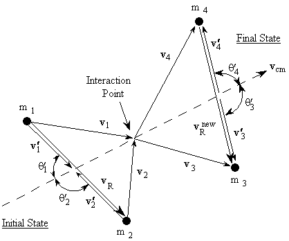
Figure 2. Two-body final state reaction kinematics

The kinetic energies of each particle are labeled in the plasma (i.e. "lab") frame as , while in the "center of mass" (cm) frame they are written as . The kinetic energies of the motion of the center of mass and the relative motion of the incident particles are related to these particle energies as follows:

and

where

The kinetic energy associated with the relative motion of the exit particles is

where

and

We assume that the quantities M (= m₁ + m₂ = m₃ + m₄), T_cmand v_cm are the same before and after the interaction, within a very small error (of the order of Q/Mc² where M is the total reaction particle mass), and that the relative velocities v_R and v_R^new are each independent of frame of reference.

We calculate Maxwellian-averaged mean properties of these reaction quantities by first expressing all energies in terms of T_R and T_cm, since, as we will show, this facilitates developing the separable expressions for their statistical averaging. This transformation, however, has a much deeper significance apart from this convenient consequence, because it effectively separates the plasma-related phenomenology and the nuclear interaction. This is because in any interaction in the plasma, the center of mass motion v_cm and the relative particle motion v_R are independent of one another, i.e. uncorrelated. Thus the center of mass kinetics are determined solely by the plasma properties, and none of the nuclear interaction properties depend on any of the center of mass quantities — including the direction of v_cm. And, s is a function of T_R and not of T_cm. This is why — as we will show later — the statistical average of T_cm depends on q, that for T_R depends on both q and s, and the angular correlations between relative and center of mass motion quantities average to zero.

We first express the initial particle velocities in terms of v_R and v_cm, as follows:

From this we see that v₁¢ = m₂v_R/M and v₂¢ = - m₁v_R/M. It is then a fairly straightforward procedure to use the previous definitions of the various kinetic energies to obtain the initial state energies and relations in terms of T_cm and T_R:

and

where the q_i¢ are the angles that v₁¢ and v₂¢(and therefore v_R) make with v_cm, as shown in Figure 2. In other words,

where the caret ( ˆ ) denotes the unit vector.

The final state particle energies and relations are correspondingly rendered, when it is understood that the reaction Q-value (the energy released by the reaction process) is included only in the final particle energy and velocities, and leaves the center of mass quantities T_cm, v_cm and M unaffected with negligible error. This says that

is the only essential difference; thus the relations for the final state can be copied directly from those of the initial state by appropriately relabeling the particle indices. We then have that

and

q₃¢ and q₄¢ are the angles that v₃¢ and v₄¢(and therefore ) make with v_cm, as shown in Figure 2, so that

We can now address the statistical average of these reaction energies and cosines over the plasma distribution, and this requires some care. Basically, the only way to obtain the mean value of a reaction quantity in a plasma is to calculate its average over a reaction probability distribution, and the only distribution that qualifies is the reaction rate function that determines – not just the Maxwellian distribution of the plasma. This function is the integrand used to calculate , or

which is a joint probability distribution in d³v_Rd³v_cm space. It is important to note that this function identifies, or selects, in a statistical sense, the distribution of that part of the particle population of the plasma that participates in the reaction, and only that part. It is also important to notice that this distribution identification holds for any and all final state configurations that result from the reaction, which is to say that it is independent of whatever values and directions the final state particle velocities do take. As we will show shortly, this concept is the key element that helps resolve anisotropic differential cross-section issues (Perkins, 1990 and 1991) that arise in calculating the Maxwellian-averaged reaction quantities for the final state.

Because F is not normalized to 1 (its integral is equal to ), the statistical average of any quantity, say f, over this reaction probability distribution, which we denote by , is calculated by the classic ratio of two integrals,

where the subscript "reac" on the angular brackets denotes the statistical average over the reaction distribution F, and the angular brackets without a subscript continue to denote the statistical average over the Maxwellian distribution. Thus the denominator in the above is, of course, , while the numerator is (now obviously) the Maxwellian average . We can write this more compactly as

Notice that the exponents in the integrands are T_R/q and T_cm/q, which is the reason for rewriting all kinematic quantities in terms of T_R and T_cm. This means that if the quantity f is separable into functions of T_R, T_cm (or v_R, v_cm) or the angular directions, then individual integrations over these arguments can proceed separately. As it turns out this will indeed be so for our needs.

We developed T_i in terms of T_R, T_cm and the cosines given by and . It is a fairly easy matter to obtain the reaction rate averages of these latter quantities, since their integrals are now separable. The statistical reaction average for T_R reduces to a single integral much the same way as the statistical Maxwellian average for sv worked out, and the result is

Here, too, numerical integration is required, in an equally simple form as for.

Zimmerman (2001) has pointed out that the slope of the curve as a function of q is related to . This is immediately evident by differentiation: one finds, by including the ∂ /∂q operation on the integrand, that

Thus can be expressed in terms of . The reaction statistical average for T_cm easily reduces to its Maxwellian average:

Finally, we consider the reaction averages of the particle direction cosines, which contain some subtle issues. To calculate the reaction statistical average of the cosine term , we select the direction of v_cm as the z-axis for the polar coordinate system for v_R. Then

and the angular integral part (in the v_R system) of the reaction average of this quantity vanishes:

Thus

This reiterates our earlier observation that v_R and v_cm are uncorrelated. The reaction statistical average of the cross-terms in the expressions for T₁ and T₂ therefore vanish.

Next, we calculate the reaction statistical average of the post-reaction cosine term . However, the angular anisotropy in the emission of final state products needs to be addressed, because the angular distributions ds/dW of final state particles in nuclear reactions are neither uniform nor constant. As it turns out (Zimmerman 1990) this is of no consequence, because the angular distribution is a function of the angle that makes with the initial relative velocity direction , and the direction cosine of , as we showed earlier, has a reaction statistical average of zero. We may put this in another, more graphical way. Suppose one of the final state reaction particles was emitted preferentially at some fixed angle a which makes relative to the original interaction particle direction of approach, . The statistical average would then be taken of the cosine of this direction relative to the direction of (which is the polar axis for the integration). We are therefore in fact calculating the statistical reaction average of the quantity

and this, too, results in zero. Thus the reaction statistical average of the cross-terms in the expressions for T₃ and T₄ also vanish.

The reaction statistical average of the particle kinetic energies in the plasma are thus as follows:

Energy conservation clearly still holds during reaction averaging:

We emphasize again that the statistical averages which are labeled by the subscript "reac" are over only those particles that actually participate in the reaction, and not the entire plasma population. The above conservation law is thus so restricted. Perkins and Howerton (1988) obtain the same results but with a priori initial assumptions of average energy conservation and isotropy of reaction angular distributions. Our treatment does not require these assumptions.

4. Exit particle energies in the t(t,2n)a reaction: a foray into three-body final state energy averaging

The Maxwellian-averaged mean energies of the three exit particles in the t(t,2n)a reaction are handled differently, because at any given initial particle total energy, the center-of-mass energies of the exit particles are distributed, rather than sharply clustered at a single value. This is because this reaction proceeds partly by instantaneous three-particle breakup, and partly by a sequence of two-body states. In the latter process ⁵He is formed by the t(t,n)⁵He reaction, and then breaks up into a neutron and an alpha while in flight.

In the current version of the TDF system, we estimate the mean energies of the exit particles in the center-of-mass frame for the t(t,2n)a reaction by calculating the expectations of their energies over the final state energy distributions that were experimentally measured at LLNL by Wong, Anderson and McClure (1965). They directed a 500 keV beam of tritons on a tritium target and measured the energy spectrum of the neutrons and alphas emitted perpendicular to the beam line. The resulting center-of-mass frame neutron and alpha energy distributions suggested that the t(t,2n)a reaction proceeded 70% by direct three-body breakup, and 30% by sequential two-body final states, first by the t(t,n)⁵He reaction, then by breakup of ⁵He in flight into an alpha and a neutron. The 30% sequential breakup distribution was further estimated to subdivide into two competing processes in which ⁵He was either left in the ground state (20% of the time) or in a broad first excited state at 2 MeV (10% of the time). (This first excited state has subsequently been assigned a level energy of 4 MeV, see Ajzenberg-Selove (1988)). Each one of these three processes (channels) results in different mean energies for the two neutrons and alpha particle. The mean energies of these particles for all reaction processes are therefore their expectation energies, which are the sum of their mean energies in each process weighted by the relative frequency of each process.

If we make the simplifying assumption that these branching ratios hold for the t(t,2n)a reaction in a warm plasma, then the mean energies of the exit particles can be approximately modeled in a relatively straightforward manner. We first consider the reaction kinetics at zero plasma temperature, for then the center-of-mass frame is at rest and the emitted particle energies take on simple and well-defined distributions. In the simultaneous three-body breakup process, the exit particles each have a phase space spectral energy distribution of the form

where

M is the sum of the particle masses, and i = 3, 4 and 5. (This corresponds to the two neutrons and one alpha particle of the t(t,2n)a reaction). The average of the particle energies over this symmetric distribution is obviously

In the sequential two-body final state mode, the first final state is the "usual" two-body case, and the energies of the emitted particles are

for i = 3 and 4 (corresponding to the neutron and ⁵He nucleus of the t(t,n)⁵He reaction). Their energy distributions are very sharp, so for i = 3, 4. The second final state occurs when the heavier particle (say, m₄) breaks up in flight into two particles, say m₅ and m₆ (corresponding to a neutron and an alpha particle), and releases breakup energy Q_B in the process. The exit particles in this stage have a uniform (boxcar) distribution of energies between two limits, which are given (for, e.g., particle 5) by the relations

The average particle energy over this distribution is evidently

For the t(t,2n)a reaction, the Q value is 11.33 MeV, and there are two known competing sequential two-body final states corresponding to ⁵He left in the ground state and in a broad first excited state at 4 ± 1 MeV (Ajzenberg-Selove, 1988). The breakup energy (Q_B) for ⁵He in the ground state is .89 MeV, and for the first excited state it is approximately 4.89 MeV. The mean particle energies (i.e. the average over that particle energy distribution) for each channel of this reaction are calculated from the above expressions, and the results are presented in the following Table I.

channel and fraction (b_i)				E_x(⁵He)
three-body breakup (70%)	4.718	4.718	1.906	-
1^st sequential two-body (20%)	8.694	1.066	1.589	0
2^nd sequential two-body (10%)	5.363	4.124	1.854	4 ± 1
weighted mean, 3 channels	5.577	3.928	1.838	-

Table I. Mean center-of-mass frame energies (MeV) for

t(t,2n)a exit particle distributions in each channel

The last line in the table gives the weighted mean energies of each particle over all reaction channels. These are calculated from their expectation sum, which is

where the subscript i is the channel label, is the particle energy for each channel averaged over the particle's distribution, and the branching ratio fractions b_i for each channel (also given in the table) sum to unity: b₁ + b₂+ b₃ = 1.

We estimate the reaction-averaged energies of the three exit particles as a function of plasma temperature by the following model, which is used in the TDF system until a more comprehensive and correct treatment of three-body final state energetics in a warm plasma is developed. The three weighted mean center-of-mass energies in the table add up to the final state total kinetic energy, which is the Q value. This corresponds to a plasma at zero temperature. The partition fraction that each exit particle i has of this total energy is f_i = /Q, so for the three particles we have f_n1 = 0.492 ± .007, f_n2 = 0.347 ±. 007 and f_a = 0.162 ± 001. The uncertainties are due to the ± 1 MeV uncertainty in the energy level of the first excited state of ⁵He. We now assume in our approximation model that these same fractions f_i (of the reaction-averaged final state total energy) also determine the reaction-averaged energy of the exit particles for any plasma temperature (White, 1990). That is, for any given q we calculate for each exit particle i, where

and where subscripts 3, 4 and 5 correspond to n₁, n₂ and a. Then the reaction-averaged mean kinetic energies of each exit particle are assumed to have the values = 0.492 , = 0.347 , and = 0.161 at that plasma temperature.

The procedure is thus to first calculate for a given q, and then use the above partition fractions to estimate the three final state particle values. These fractions are "hard-wired" into the TDF system mean energy lookup routine for the t(t,2n)a reaction. It is expected that these averaged energy estimates — as derived from the partition fractions — will be revised (perhaps minimally) when a correct three-body final state reaction formalism is eventually developed for the TDF system.

The t(t,2n)a reaction partition fractions used in earlier versions of the TDF system differ slightly from the ones given above: they are f_n1 = 0.473, f_n2 = 0.364,and f_a = 0.163. The reason for this is that a final state consisting of three sequential two-body final state channels was used to calculate the partitioning, and the three-body breakup mode was not considered. The ⁵He nucleus was assumed to have its first and second excited states at 4 and 8 MeV, so that three channels corresponded to the ground, first and second energy levels. These channels were each assumed to occur with an equal probability of 1/3. These older partition fractions appear close enough to the correct ones to have caused little error in their use.

5. Maxwellian-averaged two-body final state reaction particle spectra

In the center of mass system of two reacting nuclei the kinetic energies of each particle are given by T₁¢ = m₂T_R_/M and T₂¢ = m₁T_R_/M where T_R = T₁ + T₂ - T_cm. If the final state contains two particles, their center-of-mass energies are then, just as simply, T₃¢ = m₄(T_R +Q)_/M and T₄¢ = m₃(T_R +Q)_/M. In the limit of a very cold plasma (i.e., q @ 0) the kinetic energies of these exit nuclei would be T₃¢ = m₄Q_/M and T₄¢ = m₃Q_/M. Such energies are sharply defined, and diagnostic measurements would show them to have a very narrow energy spread. In progressively warmer plasmas, i.e., as q increases, the energy spread around these values and the centroid of the distribution also increases; each final state particle energy becomes distributed over some energy range, and thus develops into an energy spectrum that is characteristic of the reaction and the plasma.

In this section we outline a practical analytic integral approach to deterministically calculating this energy spectrum for a thermonuclear reaction in a Maxwellian plasma, which is used in the TDF system. This approach was reported by Williams, and much of the development which follows was taken from his paper (Williams 1971). Williams defines a "super-distribution" for two-body final state nuclear reactions in a plasma with a function f(v₁,v₂,v₃,v₄), which measures the probability that the reaction has occurred in such a way that the initial two particles have vector velocities v₁ and v₂, and the final two particles have vector velocities v₃ and v₄. Then the probability that the reaction does occur at all — for any values of v₃ and v₄ — is necessarily given by the following integral result:

where s is the total reaction cross-section corresponding to the initial two particles having the velocities v₁ and v₂ (or relative velocity v_R = |v₁ -v₂|). To ensure conservation of energy and momentum in the reaction process, Williams redefines f(v₁,v₂,v₃,v₄) by implicitly defining a new function g(v₁,v₂), as follows:

This form is substituted in the above integral and the integration carried out, making full use of the d function properties. This results in the following "normalization function":

When the above expressions for s, f and g are combined, we have a redefined form for s to insert in the integral which formally defines , which is

or, a little more explicitly,

We now employ a useful short cut developed by Williams: we "unpeel" from this multiple integral the presumed rate of production of final state particle 3, by formally omitting the integration over d³v₃ to obtain the distribution

This is formally equal to the number of particle 3's produced in the reaction with velocity v₃ within cell d³v₃in velocity space; the integral of n₃d³v₃ recovers the full statistically averaged reaction rate . It is also clear that n₃ contains the spectral information associated with the plasma and its distribution functions f(v_i). We bring this out more explicitly by noting that the directivity in the production of particle 3 in the plasma is isotropic; the basis for this assumption was presented in Section 3 and is discussed more fully at the end of this section. Then the angular part of the integral of can be carried out with the result that

Because dT₃ is the integration element, we can identify the last integrand as the spectral energy density of reaction product particle 3 in the plasma; it is the number of particle 3's produced with energy T₃ in the interval dT₃ per unit volume per unit time. Thus the particle 3 spectral rate density is

This is the formal expression of the energy spectrum of the emission of particle 3 in the isotropic plasma. The evaluation of the integral for n₃ results in the explicit numerically integrable expression for the energy spectrum dN₃/dT₃ of particle 3 as a function of its energy. The full formal expression of the integral for dN₃/dT₃ is therefore as follows:

where we have replaced the general plasma particle distribution functions f(v_i) by the Maxwellian forms f(m_i,v_i,q), as given previously in Section 2.

We sketch here only briefly the procedures we used to reduce this formidable integral. We first express all velocities in terms of v₃, v_cm, and v_R, and then carry out the integration over d³v₄, utilizing the momentum d function in the process. Two integrals result, with v_cm and v_R as the variables of integration. which are not totally separated because the energy d function argument contains both variables. However this argument does contain the cosine of the angle between v₃ and v_cm, so the angular part of the v_cm integral is evaluated using v₃ as the z-axis, while "using up" this d function. Then the integration is carried out over v_cm. The "final result", representing much algebra and evaluation of the energy d function over finite angle limits (see Appendix C), is a single integral over the variable T_R, as follows:

where the exponents are given by

The functional dependence of dN₃/dT₃ on T₃ is now clearly evident. In fact, if we integrate dN₃/dT₃ over dT₃ we indeed recover , as we should. (This integral was also presented by Talley and Hale (1988) but without elaboration.)

Because of particle symmetry in the equations, we obtain the spectral energy distribution for particle 4 from the above merely by switching labels 3 and 4 in all of the preceding derivation. dN₄/dT₄ is obtained, as it were, "by inspection."

Note that the exponents in the above integral can be rewritten as

and since v_cm = v₃ - v₃¢ we can have, alternatively,

corresponding to the cases where v₃ and v₃¢ are parallel or antiparallel, respectively. Also, and as defined above are the limits for the integration over dT_cm , which in turn come from the angular integration of the energy d function over the direction cosine of v_cm, or cosq_cm. This angular integration is carried out by the steps shown in Appendix C.

We close this section with the resolution of a subtle and historically persistent issue. Our definition of the f and g functions given above was taken from Williams (1971) and contains the total cross-section s rather than the differential cross-section ds/dW. This implies a priori that the details of the reaction angular distribution do not affect particle spectra. Heinrichs et al (1989) included this angular distribution explicitly in their formulation, and obtained an integral for the particle spectra similar but not identical to Williams'. Their spectrum integral also contains s, and they assert that it depends in no way on the angular variation of ds/dW. Perkins (1990) addressed this angular anisotropy issue by carrying out Monte Carlo calculations of two-body final state energy distributions for reactions having markedly non-isotropic differential cross-sections ds/dW. He found empirically that the angular variation of ds/dWhad no effect on the final state particle spectra.

This anisotropy issue is actually moot. We observe that s rather than ds/dW occurs in all joint distribution functions treated here, because s is the probability for the thermonuclear reaction to occur at all. It therefore selects, as it were, only that subset of the particle population in the plasma that participates in the reaction, and it thereby defines the reaction distributions. This selection is independent of final state properties, that is, it holds for any final state configuration that can occur. At no point does the angular distribution of the final state particles become a factor. Both F in Section 3 and g(v₁,v₂) in this section have this independence property. The angular properties of the final state in the Maxwellian plasma — which is inherently isotropic to begin with — are determined by the conservation laws, and these are put into effect by the delta functions in the integrand of the spectral distribution functions dN_i/dT_i. The statistical reaction average of the direction cosines as treated in Section 3 also vanishes for this same reason.

6. Digression on two-body final state spectrum moments

The integral defining the two-body final state spectrum distribution dN₃/dT₃ can be used to work out the moments of this distribution directly without actually evaluating it, because the exit particle energy T₃ appears only in the part of the integrand which is the difference of two exponentials. The general integral for the n^th moment of the spectral distribution is the spectral expectation average of , or

The actual integral over dT₃ that is needed to work out these moments is

where a(±) is as given in the previous section. This integral I_n is used to evaluate both the numerator and denominator of the expression for because, evidently,

and the case n = 0 applies to the denominator. Although the multipliers in front of the integrals can cancel out in the ratio, they are not discarded here.

There exist different algebraic approaches for evaluating these auxiliary moment integrals I_n. The one we use is to first make the substitution and rewrite the integral in the form

where and . We reconsider this as the difference of two separate integrals I_n = I_- - I₊ where the new ones are

These integrals are simplified further by making the substitutions u = x + b in I₊ and u = x - b in I_-. The results are

and

When these two integrals are subtracted, the finite integrals combine to zero, leaving the result

This reduces (for any given n) to well-known definite integrals when the difference term is expanded and simplified further.

We are interested particularly in I_n for the cases n = 0 and n = 1, which evaluate to

and .

Higher moment integrals may be evaluated similarly. On replacing a and b with their original meanings, carrying out algebraic reductions, and inserting the results appropriately in the moment integrals, we find – as we asserted earlier – that

which is the denominator of . It is also the numerator for the zeroth moment and the area under the spectrum distribution curve dN₃/dT₃. Straightforward algebra then produces the following result for the first moment of the spectrum distribution:

where is as given in Section 3. In other words, the zeroth spectrum moment is obviously unity, and the first spectrum moment is the reaction statistical average of the final state particle kinetic energy T₃. This is to be expected: the first moment of a distribution is the mean. Thus we have evaluated the mean exit particle energy by explicit use of the exit particle spectrum distribution. These spectrum average results were also derived by Williams (1971).

7. Data, algorithmic bases and results of calculations

The Thermonuclear Data File (TDF) system as currently implemented uses the cross-section data for five exothermic hydrogen and helium nuclear reactions, which are listed with their Q values as follows:

d(d,n)³He Q = 3.26891 MeV

d(d,p)t 4.03271

t(t,2n)a 11.3321

t(d,n)a 17.5894

³He(d,p)a 18.3532

In Figure 3 we show log-log plots of the total reaction cross-section s(T_R) for each of these reactions as a function of the relative kinetic energy T_R of the two initial particles in their center-of-mass system, from about 100 eV to 15 MeV. This laboratory frame cross-section data was provided by the LLNL Nuclear Data Group (White, 1990). These are the cross-section functions that are used in all integration procedures described in this report.

Because of the smoothness of these data in log-log space, all interpolations and lookups on these cross-sections are carried out by the cubic Lagrange technique, which provides extremely smooth and highly accurate results even though logarithmic and exponential operations are used. The cubic Lagrange interpolation procedure fits a cubic in Lagrange form through four points, and then the interpolation is carried out between the two inner points. The Lagrange interpolating cubic function has the following form:

f(x) =

f₁(x - x₂)(x - x₃)(x - x₄)/((x₁ - x₂)(x₁ - x₃)(x₁ - x₄)) +
f₂(x - x₁)(x - x₃)(x - x₄)/((x₂ - x₁)(x₂ - x₃)(x₂ - x₄)) +
f₃(x - x₁)(x - x₂)(x - x₄)/((x₃ - x₁)(x₃ - x₂)(x₃ - x₄)) +
f₄(x - x₁)(x - x₂)(x - x₃)/((x₄ - x₁)(x₄ - x₂)(x₄ - x₃))

where f₁, f₂, f₃ and f₄ are the values of the interpolant data at the points x₁, x₂, x₃, and x₄. In the case of the cross-section data in the TDF system we use ln s(T_R) for the f_i and ln T_R for the x_i. The four adjacent ln T_R entries in this array used to construct the cubic are chosen so that the interpolating point lies between the middle two. The LLNL cross-section file energies are spaced so that linear interpolation of the cross-section as a function of energy is accurate to within 1 %. Using the cubic Lagrange procedure on this array in log-log space in the manner just described can provide an interpolation accuracy of the order of 10^-⁵, i.e. .001 %.

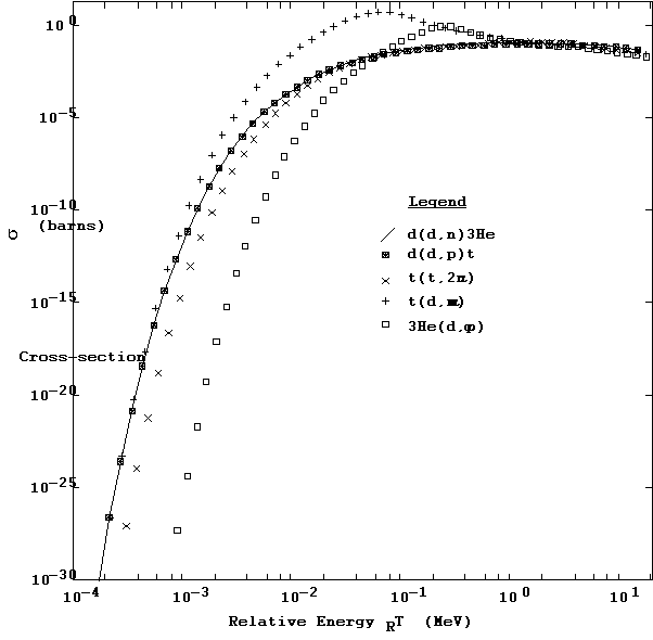
Figure 3. Total cross-section for five TDF reactions

The Gamow function integrands for the Maxwellian-averaged reaction rates are similarly smooth, and typical cases are shown in Figure 4 for — by way of example — the t(d,n)a reaction at three different Maxwellian plasma temperatures. The cross-section function for this reaction — which is part of the integrands — is also displayed for comparison.

These integrand functions are displayed again in Figure 5 in a linear-linear plot, but this time renormalized to the same peak value, in order to show off differences in form and width for different plasma temperatures. From Figures 4 and 5 it is seen that the maximum contribution to the integral comes from progressively larger values of s and T_R as the plasma temperature qincreases.

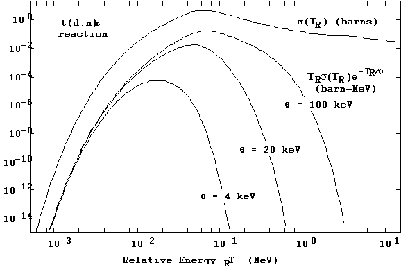
Figure 4. Gamow integrand functions and cross-section data

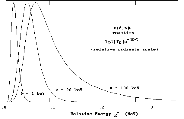
Figure 5. Linear-linear plot of Gamow integrands.

The integration procedure used to calculate is illustrated schematically in Figure 6. For a given temperature q, the energy T_R and value at which the Gamow integrand function peaks is determined by table lookup, and the two values of T_R at which the function is at 10^-⁴ of this peak are calculated by Newtonian root iteration. These two values (and ₎ determine three integration intervals. The integration over the middle (main) interval between and is carried out by one or two 16-point Gauss-Legendre quadratures, depending on the interval size. The integration from 0 to is done by fitting a power law function of T_R to the integrand over this interval, and integrating that function. The integration from to ∞ is done by fitting an exponential in T_R to the integrand over that range, and integrating that function. The integral for is then the sum of these three integration results. The accuracy of this approach has been verified to six places by using it to evaluate integrals of t^z^-¹e^-^tdt and t^-ⁿe^-^ztdt, and comparing answers with published values of the Gamma function G(z) and exponential integrals E_n(z). (The integral of was also accurately evaluated as a special case of E_n(x).)

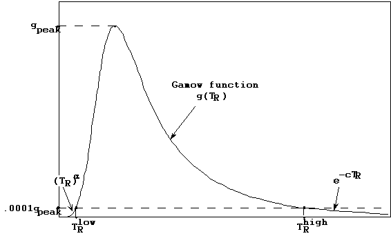
Figure 6. Gamow function integration intervals

There are three other practical reasons for preferring this algorithmic approach to the integration. First, only the relevant range of the integration variable T_R is used, as opposed to doing the numerical integration over the entire data range; the integration is thus efficient and also minimizes computational noise. Second, this integration procedure is well-suited to the other Maxwellian-distribution type integrals required for the TDF system, and is also used for them. Third, this integration technique is extremely fast, and permits function lookups and iterative root findings by direct integration, rather than by interpolation over pre-calculated arrays. It thereby facilitates accurate numerical double integration required to generate the output particle energy spectrum quantities.

The results for the reaction rate integration for the five TDF system nuclear reactions are shown in Figure 7, in which is plotted as a function of the plasma temperature from 1 keV to 1 MeV for each reaction. As with the cross-sections, the reaction rates also range over several orders of magnitude.

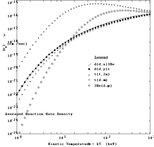
Figure 7. Reaction rate for five TDF reactions as

a function of the plasma kinetic temperature.

Previous calculations of have been carried out by many authors. The ones done at LLNL prior to the current TDF system have been reported by Greene (1967) and Howerton (1979). The generation and use of in stellar nucleosynthetic and other astrophysical contexts is outlined, for example, by Caughlan and Fowler in their 1988 compilation and earlier papers.

8. Algorithmic bases and results for , and

The Maxwell-averaging integrals used to calculate the mean particle energies and final state spectra are evaluated in the same manner as for the reaction rates; the integrands are morphologically identical. In Figure 8 we show — using the d(d,n)³He reaction in a 100 keV plasma as an example — the functional forms of the integrands for the reaction rate , the mean relative initial state kinetic energy (which is used in obtaining all the ), and the Maxwellian-broadened energy spectrum for each final state particle. The integration procedure for the Gamow function described in Section 7 and illustrated in Figure 6 applies equally well to these other integrands.

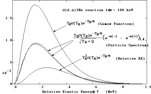
Figure 8. Integrand function forms for the Maxwell-averaging procedures,

using the d(d,n)³He reaction in a 100 keV plasma to create this example.

For the Maxwellian averaged mean particle energies only the averaged values of T_R and T_cm are required since the are linear combinations of and = 3q/2, and is the only average requiring an integration. Example results are shown in Figure 9 as plots of , and the for i = 1, 2, 3, 4 versus plasma temperature q, for the d(d,p)t reaction, where q ranges from 0 to 1000 keV. The indicial correspondence here is that particles 1 and 2 are d's, particle 3 is a p and particle 4 is a t. For the most part these variations are fairly linear in q (and is exactly linear). Indeed, one could approximate ≈ 2q for this reaction. Note that the values of and at zero temperature correspond to m_iQ/(m₃ + m₄) for i = 4 and 3 (where Q ≈ 4 MeV), as they should.

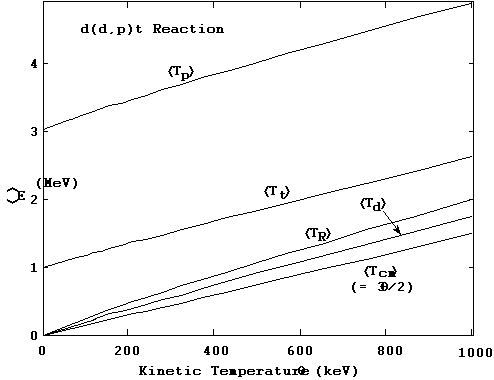
Figure 9. Maxwellian averaged mean particle and system energies

for the d(d,p)t reaction as a function of plasma kinetic temperature.

The integrations for the reaction rate spectral distributions dN_i/dT_i are likewise straightforward, and handled the same way as the other integrations just described. We show in Figures 10a and 10b the final state energy distributions calculated in the TDF system for the two exit particles in the d(d,p)t reaction. The log-log plots in 10a indicate the stability the TDF integration procedures are capable of, as they show how well the regularity and smoothness of the spectrum functions are maintained over several orders of magnitude.

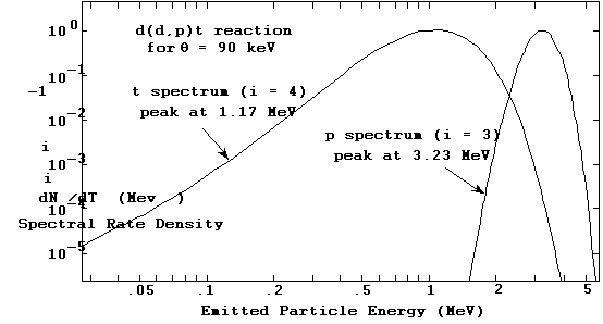
Figure 10a. Final state reaction rate spectral density distribution

for the d(d,p)t reaction at a plasma temperature of 90 keV.

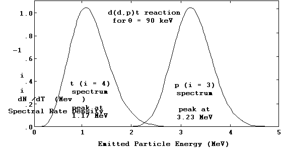
Figure 10b. Final state reaction rate spectral density distribution

for the d(d,p)t reaction at a plasma temperature of 90 keV.

We need to point out that the energy averaging and spectral calculation procedures just described apply only to those TDF system reactions that have two-body final states; the t(t,2n)a reaction, with three particles in the final state, is handled differently. For this reaction no spectral information is provided, as this requires development of three-body final state spectral distributions and their adaptation to thermonuclear plasmas. This will be the subject of a separate and forthcoming report. The reaction-averaged mean energies of the final state particles in the t(t,2n)a reaction, however, are calculated using the approximate multiple channel model developed earlier in Section 4.

9. Algorithmic basis of the final state spectral probability distributions

One of the main uses for final state spectral distribution information is to provide a probabilistic basis for final state configuration sampling in Monte Carlo simulations involving plasma reaction products. The integral over the final state spectral distributions, when treated as a function of the spectral energy, can be used for Monte Carlo sampling. Recall that dN_i/dT_i is the final state particle spectral distribution function for some particular output particle for a given reaction in a plasma at a given plasma temperature, viz. i = 3 or 4 (or even 5). Let us define a normalized spectral distribution by the function

Then the integral of this normalized distribution as a function of energy is given by

Because the area under the spectral distribution dN_i/dT_i is indeed , this monotone integral function is asymptotically bounded on [0,1], that is, I_i(0) = 0 and I_i(∞) = 1. It is therefore suitable for the random statistical sampling over [0,1].

It is very useful to define an auxiliary function u_i(T_i) by the relationship

This is inverted to obtain the following defining functional form for u_i:

We also find that an equally convenient relationship defines S_i in terms of u_i and its first derivative, as follows:

We show in Figure 11 plots of these three functions for the third particle (the neutron) from the t(d,n)a reaction, at a plasma temperature of 90 keV. The display is in three parts, one for each function, with a common energy abscissa.

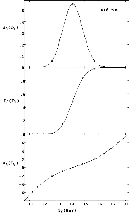
Figure 11. Spectral, probability and auxiliary functions for the

neutron output from the t(d,n)a reaction at 90 keV.

The reasons for using the (1 + tanh) function to reformulate I_i(T_i) are, first, that I_i(T_i) has roughly that form, and, second, the auxiliary variable u_i provides a very convenient basis from which to do extremely accurate interpolation over a small collection of points that define the values of S_i and I_i as a function of T_i. The way this works in the TDF system is as follows: when an input random number value for I_i is provided, the corresponding u_i is determined by calculating u_i as a function of I_i. Then we interpolate both du_i/dT_i and T_i at this u_i and obtain S_i. The convenience of this arrangement stems from the fact that T_i and u_i are very smooth functions of each other over the entire practical energy range, and so the other quantities can be very accurately interpolated — over many orders of magnitude in spectrum amplitude — with very few points. This smoothness appears to be present for all reactions and particle output types in the TDF system. To show the power of this procedure, we used only the 11 points indicated by small squares in each of the first two graphs of Figure 11 to interpolate from, and thus generate all three curves shown.

It is clear that generating the data for the cumulative probability distribution I_i(T_i) requires numerical double integration, and we detail how this is done in the TDF system. For each spectrum at a prearranged given plasma temperature, we chose 11 points on the spectrum curve — at the peak spectrum amplitude and at the spectrum amplitudes at 0.6, .1, .01, .001 and .0001 of the peak value — to be used for the interpolating point set. The particle energies for each of these lower spectrum amplitudes are determined by using Newton's iterative root finding method on each side of the spectrum peak. In using this method every lookup of a spectrum point was done by actually carrying out the integral for the spectrum value at each iteration (rather than by interpolation). We show in Figure 12 these 11 points for the t(d,n)a reaction at a plasma temperature of 90 keV, which are indicated in the figure by the small open squares lying on the spectrum function curve. (The 11 points shown by open squares in each of the three plots in Figure 11 also have the same significance.)

The values of the cumulative probability function I_i(T_i) at the interpolation energies T_i are obtained by numerically integrating the function S_i(T_i) between each pair of adjacent points, using Gauss-Legendre quadrature. The S_i(T_i) values needed for the quadrature are obtained by actually doing the integral for the spectrum value dN_i/dT_i at each quadrature point T_i (as opposed to doing an interpolation) and normalizing to . The double integration is thus in effect a Gaussian quadrature on the spectrum distribution function with the quadrature function values determined by Gaussian quadrature on the spectrum integrand. In this way we obtain the 11 number triplets per spectrum, i.e., S, T and I, for interpolating the particle energy spectrum S and particle energy T from the cumulative probability I at a given plasma temperature. Because of the auxiliary function u, the results of the spectrum lookups are quite accurate over several orders of magnitude. This is suggested by the regularity in the semi-log plot of S₃(T₃) in Figure 12, which follows, over the range of particle energy and amplitude shown.

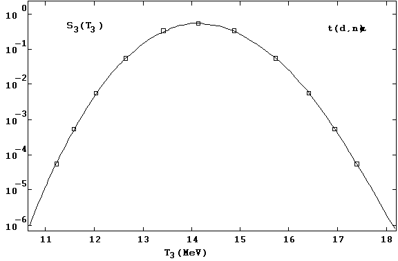
Figure 12. Calculated spectral distribution function for the

t(d,n)a reaction at a plasma temperature of 90 keV where

the interpolation array points are indicated by open squares.

10. The Thermonuclear Data File (TDF) generator

The Thermonuclear Data File (hereinafter called TDF) is the data base from which thermonuclear reaction rate and output particle spectral information are "looked up" with TDF-based subroutines, which an application code can use to read the file and generate the thermonuclear information it requires. These subroutines reside in an ASCII source code library file called TDFLIB, and are written in Fortran 77. The TDF is created by a Fortran 77 code called TDFMAKER, which carries out the mathematical and integration operations (as described in Sections 2, 3, 4 and 5) to generate data for each reaction and final state particle in the TDF system. This data is placed in the TDF in a particular standard format for lookup operations. In this section we outline briefly what TDFMAKER does, how it is used, and describe some of its key algorithms. The TDF and its lookup routines in TDFLIB will be described in the next two sections.

TDFMAKER requires as input a file identifying the nuclear reactions to be used, and a separate cross-section data file for each nuclear reaction. The content of an example input file is presented in Table II, which shows the identifying textual data for the five thermonuclear reactions d(d,n)³He, d(d,p)t, t(t,2n)a, t(d,n)a and ³He(d,p)a used in the TDF, respectively. Each line corresponds to a reaction. The first item on each line is the designated (unique but arbitrary) reaction identifier index. The second item is the count of the number of final state (exit) particles of the reaction. The next four (or five) items are the alphameric symbols for the incident particle, target particle and exit particles (in order of increasing A). The last item is the name of the file containing the lab bombarding energy and cross-section data for that reaction. TDFMAKER contains accurate nuclear masses of isotopes from A = 1 to A = 20, inclusive, and it can therefore generate the required kinematic data, including the Q-values.

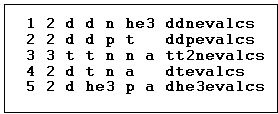
Table II: Example reaction input for the TDFMAKER code.

After reading the input file with the reaction identifiers, TDFMAKER opens each cross-section file and reads in the lab frame beam energy (in Mev) and 4p cross-sections (in barns) for each reaction. The beam energy is converted to center-of-mass energy T_R. Both T_R and the cross-section s are stored internally as logarithms of their values so as to perform cubic Lagrange interpolation in log-log space. This interpolation technique has proven good to about 5 to 6 significant figures in this application.

TDFMAKER generates the data for the TDF one reaction at a time, and keeps the generated data for each reaction in separate blocks in the TDF. After the cross-section data is read in and processed, the value of T_R for the peak of the Gamow function (i.e., the integrand) is calculated as a function of plasma temperature, since it is used to help determine the three integration intervals of the numerical integration procedure as depicted in Figure 6. In what follows we discuss how TDFMAKER is set up to calculate the integrand peak and the three integration intervals.

Gamow's model of Coulomb barrier penetration accounts very well for the non-resonant variation of thermonuclear reaction cross-sections at very low energies (Evans, 1955). It is used here to estimate the T_R at which the integrand peaks, and to provide an algorithm for the initial estimate of the numerical integration intervals. A well-known form of these cross-sections which includes Gamow's model is written as

where S is a slowly varying function of T_R that is very nearly constant at keV energies,

is the Gamow constant, a = 2π e²/hc = 1/137.03604 is the fine structure constant, c is the speed of light, h is Planck's constant, e is the electronic charge, and the Z's and m's are the charge numbers and masses of the reacting isotopes (Evans, 1955). The argument of the exponential is, of course, dimensionless. In the stellar physics field, S(T_R) is referred to as the astrophysical S-factor (Chiu 1968, Clayton 1968) and is generally tabulated in cross-section data for stellar nucleosynthesis. Here, for each reaction, we take S to be a constant which normalizes s_G(T_R) to the reaction s(T_R) at low energies. In Figure 13 we plot the cross-sections s(T_R) for each reaction, with the corresponding Gamow model cross-section s_G(T_R) plotted superposed.

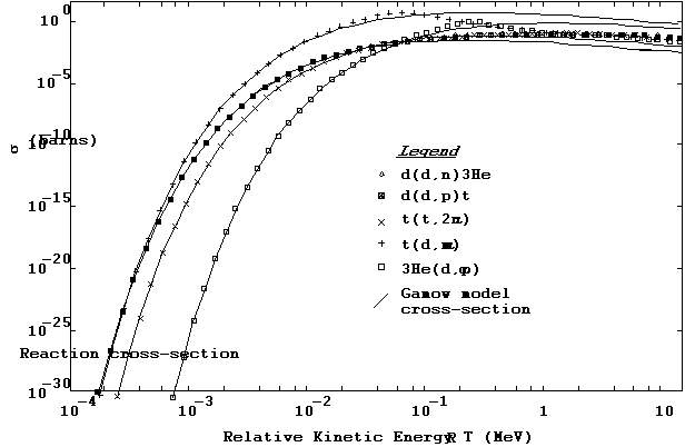
Figure 13. Reaction cross-sections: actual data and

corresponding Gamow analytic model s_G for each reaction.

At low energies the fit of s_G to the various s's for each reaction is excellent, but deteriorates at the higher energies. To ensure accurate determination of the T_R of the peak over all data energies, we use a "variable Gamow constant" scheme in TDFMAKER in which g is calculated at each energy point T_R(i) of the cross-section array s(i) so as to make s_G fit the data in the neighborhood of that T_R. Thus we estimate the "local" value of g at the i^th point of the cross-section array as follows:

It is worth mentioning that for all five reactions currently used in the TDF system, g(i) as a function of T_R is approximately constant up to about T_R = 100 keV, after which it varies significantly with higher values of T_R.

When s_G is used in place of s, the integrand takes the following form:

To find the value of T_R at the peak of this function we set ∂G/∂T_R = 0 and regard S and g as constants. This results in the following power law relationship between T_R of the peak and the kinetic temperatureq:

This recipe (i.e., the power law formula using data-fitted "variable" g) is an excellent peak finder for the Gamow integrand, as shown in Figure 14 for the d(d,p)t reaction and in Figure 15 for the t(d,n)a reaction, where we present a log-log plot of q versus T_R at the peak for these reactions in three different ways. The curved line represents the power law with the "variable" recipe for g. The straight line represents the power law with g fixed at Gamow's constant. The symbol ¥ locates the value of T_R at which the integrand array calculated for the plasma temperature q actually peaks. The "variable g" recipe appears to provide the best peak predictions, while the "constant g" case does well only at lower values of T_R and q.

The data for the d(d,p)t reaction shown in Figure 14 follows the "constant g" power law relationship fairly well over most of its range, but the peak T_R values for the t(d,n)a reaction seem to approach an 80 keV asymptote, as shown in Figure 15. (This asymptotic behavior of the peak T_R is also evident in Figures 4 and 5.) The reason for this is that the cross-section for the t(d,n)a reaction has a pronounced resonance which carries over into the integrand behavior. Because the TDF system is intended for other reactions which may or may not have resonances, the variable g recipe as given above is included in the TDFMAKER algorithmic lexicon as a permanent feature. This feature and the subsequent integration limit determinations underlie most of the integrations that TDFMAKER carries out, which is the reason why a detailed description of it is included in this report.

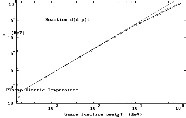
Figure 14. See text for details.

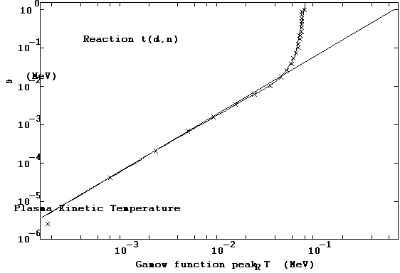
Figure 15. See text for details.

Given, then, that has been determined for a specified q, we use the Gamow function G(T_R,q) of the integrand to determine a first estimate of the two integration interval limits shown in Figure 6. Let e be the fraction of the integrand peak value at which these limits occur, and denote by T_R^* the values of T_R which we estimate by this model to occur at these limits. These are computed by determining the values of T_R^* for which the equality

holds. Taking logarithms of both sides gives the algebraic equation

This is a cubic in the variable . Rather than solve a cubic, we approximate the two solutions we need, because at low T_R^* the quantity g/is dominant, while at high T_R^* the quantity T_R^*/q dominates. Let the right-hand side of this equation be symbolized by q. Then g/ = q defines and T_R^*/q = q defines , and we therefore have

and

and are as depicted in Figure 6, where we recall that the three integration intervals are 0 to , to , and to ∞. In TDFMAKER, e has the value 10^-⁴, and the coding has checks to make sure that and indeed bracket . These interval estimate algorithms are applied to all the Maxwell-averaging integrals. When this is done, the inner interval limits are further refined by iterative root finding to be at 10^-⁴ of the peak of the integrand.

Recall next that the integrals of the spectrum function dN_i/dT_i leading to the cumulative probability functions I_i(T_i) are carried out over adjacent particle energy intervals, as outlined in Section 9. Accurate first estimates of the energy at which the spectrum function peaks and the energies bounding each integration interval can be obtained by use of the exponential difference term in the dN_i/dT_i integrand, which is given by

where i is the index label (3 or 4) for the particle of interest, the exponents are

and j is the index label (4 or 3) for the other particle. At a given fixed plasma temperature the dependence of F_i on T_i is where the variation of the final state spectrum dN_i/dT_i with particle energy T_i originates, so F_i determines the shape of dN_i/dT_i. We also note that F_i is also the integrand for the auxiliary integral I_n discussed in Section 6 on spectrum moments.

One of the more remarkable insights that emerged during the writing of this report is the realization that F_i is a very close approximation to the shape of the spectrum, dN_i/dT_i, apart from normalization. This is because the variation of F_i with T_R is quite slow, and to a very good approximation F_i can be taken outside the integral for dN_i/dT_i. In Figures 16a and 16b (as in Figures 10a and 10b) we compare log-log and linear-linear plots of dN_i/dT_i and F_i as functions of T_i for the d(d,p)t reaction at q = 90 keV, for both exit particle types. For these F_i plots T_R is set equal to its mean value at that temperature. The closeness of the shapes of dN_i/dT_i and F_i to each other, for each particle i, is excellent. We thus obtain very accurate first estimates of the integration intervals by determining those pairs of energies T_i that make F_i equal to the fractions .6, .1, .01, .001, 10^-⁴ and 10^-⁵, since the peak of F_i is very nearly 1. However, because this approach postdates the TDF system, its implementation is planned for a future version of TDFMAKER.

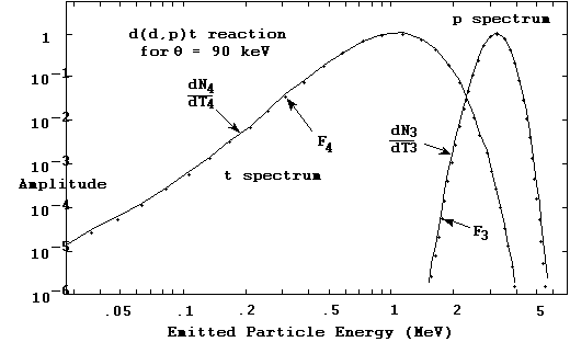
Figure 16a. Spectral distribution dN_i/dT_i (curved lines) and function

F_i (dots) for the d(d,p)t reaction at a plasma temperature of 90 keV.

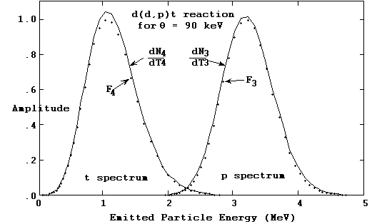
Figure 16b. Spectral distribution dN_i/dT_i (curved lines) and function

F_i (dots) for the d(d,p)t reaction at a plasma temperature of 90 keV.

The approach originally developed and currently used in TDFMAKER to determine the spectrum integration intervals is based on first inverting the preceding equation for the exponents a to obtain (for, say, i = 3)

T_R is set equal to its value T_R^peak at the peak of the integrand, because this is where the dN_i/dT_i integrand makes its maximal contribution to the integral. When a(-) is zero, a(+) is large, and F₃ is almost 1. The resulting value of T₃ estimates the energy of the spectrum peak, which we denote by . Next, when a is a large positive number, F₃ will be much less than 1, and two values of T₃ (one on either side of the spectrum peak) result, corresponding to the plus/minus signs in the parentheses. We estimate the useful energy limits of dN₃/dT₃ by setting a = ln 10⁴, so that F₃ = e^-^a = 10^-⁴, and we denote the resulting two values of T₃ by and .

In the current version of TDFMAKER, these three numbers — , , and ^r — initiate the Newtonian root-finding and peak finder procedures that determine the value of T₃ at which the spectrum peaks, and the T₃ pairs (one on each side of the peak) at which the spectrum is at .6, .1, 10^-², 10^-³, 10^-⁴ and 10^-⁵ of the peak. These procedures yield the 11 point triples (S, T and I) in the spectrum data arrays for each exit particle and each plasma temperature that are used to carry out the interpolations done in connection with Figures 11 and 12 of Section 9. It is between these values of T₃ that the spectrum functions S_i(T_i) are integrated to obtain the cumulative distribution function point values I_i(T_i).

The remainder of TDFMAKER consists of coding and algorithms to carry out the integrations, inverse lookups (root findings) and maximum findings described above and referred to in Sections 2 through 9. Two similar Fortran 77 routines in TDFMAKER were written to handle these integrations, one for the "Gamow peak integrand types" used to calculate , and the spectrum distribution dN_i/dT_i, and the other to help calculate the integrals of the dN_i/dT_i functions used for the spectrum probability distributions I_i(T_i). The first subroutine (intgrt) is a straight-forward coding of the integration scheme and limit determinations as described in the previous paragraphs. The second routine (sp3fn) is this subroutine intgrt recoded to be a function call and to carry out only the integration of the spectrum distribution dN_i/dT_i. This is so that dN_i/dT_i (in the guise of sp3fn) is used as a "callable" function within TDFMAKER, as needed. This "functionality" is what facilitates the high efficiency in carrying out the integrations over the spectrum distributions, as well as determining where the maximum of these distributions occur. Subroutine mxfnd locates the maximum of non-analytic functions by recursively fitting parabolas to point triplets and calculating the maximum of the parabola. This subroutine is used to more precisely locate the maximum of the Gamow-type integrands as well as that of the spectrum distributions.

Other Fortran 77 subroutines were developed to perform inverse lookup tasks, that is, input the value of a function and output the corresponding argument value by Newtonian root-finding techniques. In TDFMAKER the inverse lookup subroutines all have names beginning with inv. It is within these inverse routines that sp3fn is heavily used as the function value generator in determining energy arguments corresponding to final state particle spectrum distribution values.

11. Structure and content of the TDF

The information in the TDF is in alphameric format so that the TDF can be read as a plain text file. It is therefore platform-independent. The information for each reaction is arranged in separate reaction data blocks within the file, and each block has the same format, which is illustrated by the example of blocks of data from a working TDF that is shown in Appendix A. Every TDF (as of this writing) starts with a header block which is a copy of the input data for TDFMAKER (cf. Table II) that identifies the reactions and the text files containing the reaction cross-section data. Each subsequent reaction data block starts with a line labeling the version of TDFMAKER that was used to generate the block. Within each such block this line is followed by eight different types of sub-blocks of data, each starting with a header line having a unique numeric label in parentheses. The headings for each of these sub-blocks are listed in Table III.

Table III. Data block header lines in the TDF.

Heading line (1) lists the names of the files used by TDFMAKER; the last one is the name of the TDF itself. This line is followed by an alphameric identifier code which the TDFLIB subroutines check to insure that they are reading a compatible version of the TDF. Heading line (2) identifies the constants on the line which follow it, which are, respectively, the MeV energy equivalent of the atomic mass unit, the inverse of the fine structure constant, the speed of light, the Q of the reaction, and the total energies of the final state particles if those were left in excited states by the reaction. Heading line (3) identifies the nuclear masses for each particle in the reaction, in atomic mass units. Heading line (4) identifies two groups of integer data which follow it. The first five numbers are the isotope identifiers for each particle in the reaction; these identifiers have the integer value 1000Z + A where Z is the nuclear charge (number of protons) and A is the atomic number (total number of protons and neutrons). The last four numbers are respectively the number of temperature blocks for each final state particle spectrum (heading (8)), the number of lines of data in each block (heading (5)), the number of final state particles (a 2 or a 3), and the numerical index/identifier used within the TDF for that reaction. Heading line (5) identifies the data block containing the values of q, and for this reaction. Currently (as shown in Appendix A) there are 29 lines of these data triplets, each for a different plasma temperature. Also, there are 13 temperature blocks for each final state particle spectrum, where each of the 13 blocks corresponds to a different plasma temperature. Thus if there are two particles in the final state for a reaction there will be 26 spectrum blocks in that reaction section of the TDF. The 13 plasma temperatures q_i are the same for all spectrum blocks, and are equal to .0001, .001, .01, .04, .09, .16, .25, .36, .49, .64, .81, 1.00, and 1.05 MeV. The first and last temperature entries are included to preserve accuracy of the cubic Lagrange interpolation within the temperature intervals .001 to .01 and .81 to 1.00.

The remaining data blocks after line (5) refer to the output particle spectra. Heading line (6) contains the number of fractions of the spectrum peak used to define the spectrum interpolation points, and these fractions are listed in the next line. Heading line (7) identifies (for the spectrum block which follows) the plasma temperature and the final state particle index to which the block applies (a 3 or a 4 or (later) a 5), the number of lines of spectrum data, the integrated area under the spectrum curve, and the corresponding value of . (A comparison of these last two numbers gives computational diagnostic information.) Heading line (8) identifies the spectrum data block and lists, respectively, the line index j and the values of T_j, S_j and I_j for the given output particle at the temperature q_i specified. These are the actual interpolation data points used for the spectral information lookups. Currently there are 11 lines of these data quartets per block, corresponding to the peak value of the spectrum distribution and five pairs of fractional values (currently 0.6, 0.1, 10^-², 10^-³, and 10^-⁴) of this spectrum peak value. That is, S₁ = S₁₁ = 10^-⁴ S₆, S₂ = S₁₀ = 10^-³ S₆, S₃ = S₉ = 10^-² S₆, S₄ = S₈ = 0.1 S₆, and S₅ = S₇ = 0.6 S₆, where S₆ is the peak value.

As shown in Appendix A, the last five entries of I_j (i.e. index 7 through 11) in each spectrum data block are negative. This is because the numerical value of 1. was subtracted from those I_j in TDFMAKER before putting it out in the TDF, in order to retain the double precision numerical accuracy in the TDF. When these negative numbers are read in by the TDFLIB routines, the value of 1. is added to them to restore them to their original (and positive) double precision value. (TDFMAKER and TDFLIB currently declare double precision for use with 32-bit processors.)

12. The TDFLIB subroutine library

TDFLIB is the name of an ASCII Fortran 77 source program library file that contains 8 subroutines, one function subroutine, and specifications for 3 labeled common blocks. Four subroutines — tdfrdr, mxavlu, speclu, tdmass — and one function subroutine — svblu — are directly used by the applications code that needs the thermonuclear information. Subroutines tdclag, tdchlu, tdmchl and tdselu are specialized interpolation subroutines based on cubic Lagrange and Hermite methods that are intended to be used only by the other subroutines. The three labeled common blocks are tdfcon, tdfsvb and tdfspe; their memory allocation details are spelled out in comments in subroutine tdfrdr.

The main function of the TDFLIB subroutines is to perform monovariate and bivariate interpolations on the condensed data in the TDF, so as to retrieve Maxwellian-averaged and reaction-averaged thermonuclear energy and spectral information, as desired. In what follows, we present a brief description of these subroutines, their argument lists and their purpose, and then follow this by some spectrum data interpolation examples that demonstrate the calculationally robust nature of the TDF system over several orders of magnitude in the variables. Some of these routines were used to generate the plotted data shown in previous sections.

subroutine tdfrdr(iunit,ntr,ierr)

Reads data from the TDF into the three labeled common blocks in memory. It must be called no more than once by the application code before any other routine can be used. iunit is the logical unit number assigned to the TDF by the application code. ntr is the number of thermonuclear reactions read in. ierr is an error flag: zero means that the TDF was read and the memory allocated correctly. A non-zero return means the TDF was not read properly and cannot be used; this is a fatal error indicating that either the TDF was corrupted, or the version of TDFMAKER used to create the TDF, and the current TDFLIB, do not match.

In all the other subroutines, the quantity ierr is a returned error flag, in which zero means that the subroutine call was completed correctly. A non-zero error flag occurring for the main four subroutines and one function usually means that the input reaction or particle index, or one or more input numerical values, was improperly specified. In some cases, however, a more serious error could be indicated. The error flags are explained in the documentation for TDFLIB (White, Warshaw and Resler, 1990).

subroutine tdmass(ireac,bm1,bm2,bm3,bm4,bm5,q,ierr)

Returns purely nuclear masses (i.e. atomic mass minus electron masses and electron binding energies) and the Q-value q (in MeV) for a specified reaction ireac. The mass units are in amu where ¹²C = 12 amu.

bm1 = mass of lighter reacting particle

bm2 = mass of heavier reacting particle

bm3 = mass of lightest product particle

bm4 = mass of next lightest product particle

bm5 = zero for two-body final state reactions, else is the mass of the remaining product particle in three-body final state reactions

subroutine mxavlu(ireac,tp,sv,e1,e2,e3,e4,e5,ierr)

Returns the Maxwellian-averaged reaction rate sv (cm³/sec) and reaction-averaged kinetic energy (MeV) of the reacting and final particles for the specified reaction ireac and plasma temperature tp (keV).

e1 = kinetic energy of the first reacting particle

e2 = kinetic energy of the second reacting particle

e3 = kinetic energy of the first final particle

e4 = kinetic energy of the second final particle

e5 = zero for 2-body final state reaction or kinetic energy of third final particle

mxavlu identifies the data array index for the specified reaction, and determines the four sequential data temperatures which bracket the input plasma temperature tp. It calls tdclag to interpolate the reaction rate sv at this input temperature, and tdchlu to interpolate the mean relative kinetic energy er of the two reacting particles. From this and the plasma temperature it computes the reaction-averaged kinetic energies of all particles of the reaction, e1 through e5. mxavlu was used to generate the averaged kinetic energy data plotted in Figure 9, and was modified specifically to also output the average of T_R for the plot. (Note that er is the of this report, and the ei arguments are , correspondingly.)

function svblu(ireac,tp,ierr)

Returns the Maxwell-averaged reaction rate svblu (cm³/sec) for the specified reaction ireac and plasma temperature tp (keV). svblu identifies the data array index for the reaction, and determines the four sequential data temperatures which bracket the input temperature tp. It calls tdclag to interpolate the reaction rate over this temperature set. svblu was used to generate the reaction rate plots in Figure 7.

subroutine speclu(ireac,tp,ipart,pin,eout,sout,ierr)

speclu is an inverse particle spectrum lookup routine. Given the input plasma temperature tp (keV) and cumulative probability of emission pin (a real number between 0. and 1.) of exit particle ipart (3 or 4), it returns that particle's energy eout (MeV) and normalized spectral amplitude (i.e., relative probability) sout (MeV^-¹). The actual spectral amplitude is obtained by multiplying sout by the reaction rate. It is currently implemented for two-body final state reactions only. It returns a non-zero error flag and zero arguments if a reaction with three or more final state particles is selected.

ipart = 3 for the first product particle

ipart = 4 for the second (heavier) product particle

ipart = 5 is intended for a third product particle (not currently implemented)

speclu first checks the range of the input value of pin and returns special values of eout and sout if pin is exactly 0 or 1. For input values of pin between 0 and 1, speclu determines the four sequential data temperatures (and corresponding spectral data blocks in memory) which bracket the user's requested temperature tp. At each of these four temperatures it calls tdselu to interpolate the energy (e) and spectrum amplitude (s) at the user's specified cumulative probability input (pin). The resulting four values each of e and s are then interpolated at the user's specified temperature tp, by calls to tdchlu or tdmchl, as appropriate, and output as eout and sout, respectively. speclu was used to generate the data plotted in figures 10a, 10b, 11, 12, 16a and 16b.

subroutine tdclag(x1,x2,x3,x4,f1,f2,f3,f4,x,fval,ierr)

Cubic Lagrange interpolation routine for mxavlu and svblu. Interpolant x lies between x2 and x3.

subroutine tdselu(nnode,pfnode,ennode,spnode,p,e,s)

Spectrum-energy lookup routine for use by speclu. Input is p, returns are e and s, assuming 0 < p < 1. The formulas developed in Section 9 are used to interpolate e and s over the 11-point data set. Fitted power law and exponential functions are used to extrapolate e and s below and above this data set, respectively.

subroutine tdchlu(x1,x2,x3,x4,f1,f2,f3,f4,x,fval,ierr)

4-point cubic Hermite-Lagrange slope-value interpolation routine for mxavlu and speclu. Interpolant x lies between x2 and x3.

subroutine tdmchl(x1,x2,x3,x4,f1,f2,f3,f4,x,fval,ierr)

Mixed 4-point cubic Hermite-Lagrange slope-value interpolation routine for speclu. Interpolation is in linear space on nodes 1, 2 and 3 and in logarithmic space on nodes 2, 3 and 4. Interpolant x lies between x2 and x3.

The interpolation subroutines in TDFLIB were carefully checked for consistency and robustness before release. One such test was to generate contour plots of the bivariate functions I_i(S_i,q) and I_i(T_i,q) for the two output particle spectra (corresponding to i = 3 and i = 4) of each two-body final state reaction, and inspect them for smoothness over the entire variable range in the TDF. The spectrum data (T_i or S_i as appropriate) were interpolated from the TDF for 15 probability values I_i and 50 logarithmically spaced values of the plasma temperature q between 1 keV and 1 MeV, thus generating 750 data quartets (q, T, S, I) for each reaction and each output particle. From these quartets for each reaction we chose to generate two types of plots consisting of 15 separate curves, one for each value of I, for each of the two output particles. They are T₃ versus q^1/2 and T₄ versus q^1/2 on semi-log scales, and S₃ versus qand S₄ versus qon log-log scales. These curves are interpreted as contour plots of I.

Four such plots are shown in Figures 17 through 20 for the d(d,p)t reaction, in each of which the 15 contour levels of the cumulative probability function I_i are shown for the two functions, for each output particle. Figures 17 and 18 indicate approximately how the spectrum peak width increases with plasma temperature, where the various curves of I_i define the points on each side of the curve of the peak that are being followed. Figures 19 and 20 are double-sheeted in I_i since at each q there are two values of I_i for every S_i.

The essential point of these plots is that none of the 750 interpolated quartets coincide with any of the 143 spectrum data quartets for each reaction output particle in the TDF. Therefore, all calculations of the I_i(S_i,q) and I_i(T_i,q) functions for the two output particle spectra are done by bivariate Lagrange and Hermite cubic interpolation over the more limited plasma temperature and spectrum level data points in the TDF. The results are visually excellent over many orders of magnitude. These types of plots were used to choose and "shake down" various bivariate interpolation schemes during the code development phase. The ragged and "noisy" contours that were produced in the early coding stages were the best diagnostic that the interpolation procedures were not performing properly.

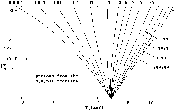
Figure 17. Contours of I₃as a function of T₃ and q for the d(d,p)t reaction.

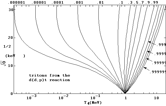
Figure 18. Contours of I₄as a function of T₄and q for the d(d,p)t reaction.

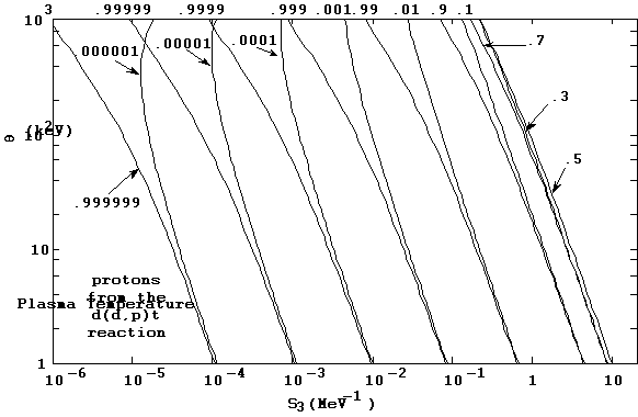
Figure 19. Contours of I₃as a function of S₃and q for the d(d,p)t reaction.

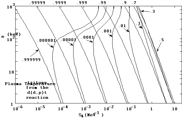
Figure 20. Contours of I₄as a function of S₄and q for the d(d,p)t reaction.

A word on the nature of the bivariate interpolation used in subroutine speclu is necessary, because it is rather specialized. Given that a plasma temperature q and a cumulative probability value I is input to a spectrum data calculation for a given reaction and a given output particle, the two spectrum data blocks at the two plasma temperatures immediately above and immediately below the input value q is are used to generate, for that input I and those four plasma temperatures q_j, four values of the spectrum amplitude S_j and particle kinetic energy T_j. These values of S and T are obtained by cubic Lagrange interpolation over the auxiliary function u that was described earlier in Section 9. For definiteness, we denote these four plasma temperatures by q₁, q₂, q₃, and q₄, in monotone increasing value, such that the input value q lies between q₂, and q₃, and we index the corresponding values of S and T similarly. The required temperature-interpolated values of S and T are obtained by modified cubic Hermite interpolation over the indexed Sand T. The way this is done is to convert the four plasma temperatures to their square root value, q_j^1/2 and then regard S_j and T_j as functions of q_j^1/2, where j = 1, 2, 3 and 4. Then the slopes of these functions are modeled at the two inner abscissae — q₂^1/2 and q₃^1/2 — by fitting parabolas to the three points at the abscissa triplets (q₁^1/2, q₂^1/2, q₃^1/2) and (q₂^1/2, q₃^1/2, q₄^1/2). This gives slopes and values for the functions S and T at the inner abscissa pairs q₂^1/2 and q₃^1/2. The cubic Hermite interpolation procedure is then carried out over these slope-value pairs to obtain the values of S and T at the square root of the input q.

Acknowledgments

The author would like to thank certain people for their assistance and contributions to the development and implementation of the LLNL TDF system described in this report. First, the late Ted Perkins, for bringing the key paper written by Williams (1971) to the author's attention, and for providing his own annotated copy of that paper to the author, with much useful commentary scribbled in the margins. Roger White and David Resler of the Physics Department's former Nuclear Data Group, for providing evaluated nuclear cross-section files and nuclear data subroutines used by the TDFMAKER code to retrieve nuclear masses and reaction cross-sections. Roger White, who, as Nuclear Data Group leader, provided a hospitable environment for development of the TDF system, and Eugene Brooks, who, as the succeeding group leader for Nuclear Data and Codes, provided support for the writing of this report now ten years later. Eugene Canfield, for indicating that the idea of conjoining the nuclear cross-section with the Maxwellian plasma distribution as the required joint distribution for the energy and spectrum averaging may have originated with John von Neumann. And, finally, it is a pleasure to acknowledge the many helpful discussions with and comments made by George Zimmerman, who took a keen interest in the development of the TDF system and its exploratory extensions to include spectra for three-body final state reactions. This report is dedicated to the memory of Sterrett "Ted" Perkins.

Bibliography and References

References to thermonuclear reaction data and modeling listed here represent neither an extensive nor an exhaustive survey of the field. Rather, they are citations of external and internal reports that the author has found helpful and suggestive in the course of developing the modeling and calculational approaches described in this report. Not all references listed were specifically cited.

F. Ajzenberg-Selove, "Energy levels of light nuclei A = 5 - 10", Nuclear Physics A490, 1 - 225 (1988)

R. E. Brown and N. Jarmie, "Differential Cross-sections at Low Energies for ²H(d,p)³H and ²H(d,n)³He", Physical Review C41, 1391 - 1400 (1990)

R. E. Brown, N. Jarmie and G. M. Hale, "Fusion-Energy Reaction ³H(d,a)n at Low Energies", Physical Review C35, 1999-2004 (1987)

H. Brysk, "Fusion Neutron Energies and Spectra", Plasma Physics 15, 611 - 617 (1973)

G. R. Caughlan and W. A. Fowler, "Thermonuclear Reaction Rates V", Atomic Data and Nuclear Data Tables 40, 283 - 334 (1988) and earlier references cited therein.

Hong-Yee Chiu, "Stellar Physics", Volume I, pp. 349 - 363, Blaisdell, Waltham MA, 1968

D. D. Clayton, "Principles of Stellar Evolution and Nucleosynthesis", Chapter 4, pp. 283 - 361, McGraw-Hill, New York, 1968

R. D. Evans, "The Atomic Nucleus", pp. 71 - 74 and pp. 874 - 878, McGraw-Hill, New York, 1955

S. L. Greene, Jr., "Maxwell Averaged Cross Sections for Some Thermonuclear Reactions on Light Isotopes", LLNL report UCRL-70522, May 1967. Preprint for paper in journal Nuclear Physics.

G. Heinrichs, et al. "Analytical Calculation of Source Energy Spectra from Maxwellian Fusion Plasmas of Arbitrary Temperature", Proceedings of the 12th International Conference on Plasma Physics and Controlled Nuclear Fusion Research, Nice, 12 - 19 October 1988, Volume 3, pp. 459 - 468, IAEA-CN-50/G-III-6, Vienna, 1989

R. J. Howerton, "Maxwell-Averaged Reaction Rates for Selected Reactions Between Ions with Atomic Mass £ 11", LLNL report UCRL-50400, Volume 21, Part A, February 1979

N. Jarmie, R. E. Brown and R. A. Hardekopf, "Fusion-Energy Reaction ²H(t,a)n from E_t = 12.5 to 117 keV", Physical Review C29, 2031 - 2046 (1984)

S. T. Perkins, "TNSPEC, a code to calculate particle spectra and energy deposition terms from thermonuclear reactions", LLNL Nuclear Data Group internal memorandum PD-61, July 1981

S. T. Perkins, "Average energy of interacting particles for thermonuclear reactions", LLNL Nuclear Data Group internal memorandum PD-62, July 1981

S. T. Perkins, "TNSP4DP, a code to calculate particle spectra and energy deposition terms from continuum thermonuclear reactions", LLNL Nuclear Data Group internal memorandum PD-72, July 1982

S. T. Perkins, "Average interaction energy of a suprathermal particle in a Maxwellian plasma", LLNL Nuclear Data Group internal memorandum PD-158, April 1988

S. T. Perkins, "The influence of the center of mass angular distribution on two-body thermonuclear particle spectra", LLNL Monte Carlo Group internal memorandum MC-10, February 1990

S. T. Perkins, "Brief comments on the center of mass system collision cosine for two body reactions on moving targets", LLNL Monte Carlo Group internal memorandum MC-12, January 1991

S. T. Perkins and R. J. Howerton, "Average Energy of Interacting Particles for Thermonuclear Reactions", LLNL report UCRL-87543. Also Nuclear Science and Engineering 82, 388 - 392 (1982)

D. R. Slaughter, "Fusion Reactivities for Several Beam and Target Ion Distributions", LLNL report UCRL-87416, September 1982. Also Journal of Applied Physics 54, 1209 - 1217 (1983)

D. R. Slaughter, "Fusion-Product Spectral Line Width in D-D, D-T and ³He-D Plasmas as an Ion Speed Distribution Diagnostic", LLNL report UCRL-97595, October 1987. Also Review of Scientific Instruments 60, 552 - 61 (1989)

D. R. Slaughter, "Effect of Ion Speed Distribution on the Spectral Shape of the 2.5 MeV Neutron Line Source Produced by DD Fusion", LLNL report UCRL-93895, February 1986. Also Review of Scientific Instruments 57, 1751 - 1753 (1986)

D. R. Slaughter, "Fusion Product Energy Spectra in Beam Heated D-D, D-T and D-³He Plasmas", LLNL report UCRL-93946, March 1986

D. R. Slaughter, "LINE: a code which simulates spectral line shapes for fusion reaction products generated by various speed distributions", LLNL internal report UCID-20374, March 1985

T. L. Talley and G. M. Hale, "Fusion Product Spectra", pp. 299 - 302, proceedings of the 1988 MITO Conference on Nuclear Data for Science and Engineering, JAERI, Japan

S. I. Warshaw, "Burning Issues in Maxwell-Averaged Reaction Rates, Probability Distributions, Data Files and Lookup Codes", LLNL Nuclear Data Group internal memorandum PD-180, Revision I, 1991

R. M. White, LLNL Nuclear Data Group, N Division, private communication (1990)

R. M. White, D. A. Resler and S. I. Warshaw, "Evaluation of Charged Particle Reactions for Fusion Applications", LLNL report UCRL-JC-107158, 7 pp. (May, 1991); Also pp. 834 - 839, proceedings of the International Conference on Nuclear Data For Science and Technology, Julich, Germany, 13 - 17 May 1991.

R. M. White, S. I. Warshaw and D. A. Resler, "Documentation for the files TDF and TDFLIB", LLNL Nuclear Data Group internal memorandum PD-179, December 1990

M. M. R. Williams, "A Generalized Energy Exchange Kernel For Inelastic Neutron Scattering and Thermonuclear Reactions", Journal of Nuclear Energy 25, 489 - 501 (1971)

M. M. R. Williams, "The Particle Spectrum from a D-T Plasma", Nuclear Science and Engineering 73, 219 - 220 (1980)

C. Wong, J. D. Anderson and J. W. McClure, "Neutron Spectrum from the T + T Reaction", Nuclear Physics 71, 106 - 112 (1965)

G. B. Zimmerman, LLNL Defense and Nuclear Technology Directorate, A Division, private communications (1990, 2001).

Appendix A. Example TDF format

-------index/input-------

1 2 d d n he3 ddnevalcs

2 2 d d p t ddpevalcs

3 3 t t n n a tt2nevalcs

4 2 d t n a dtevalcs

5 2 d he3 p a dhe3evalcs

-------------------------

TDFMKRdp version 8a of 11/12/91

(1) ddnevalcs tdfinput tdfout

8A3E911111

(2) amumev fnstnv celer qvalue exval

9.31501E+02 1.37036E+02 2.99792E+10 3.26891E+00 0.00000E-01

(3) amu1 amu2 amu3 amu4 amu5

2.01355E+00 2.01355E+00 1.00866E+00 3.01493E+00 0.00000E-01

(4) iaz1 iaz2 iaz3 iaz4 iaz5 nspec nsigv npart idreac

1002 1002 1 2003 0 13 29 2 1

(5) temp sigvb extr
1.00000E-04 1.59243E-07 1.43504E-03
1.25000E-04 2.51163E-06 1.67293E-03
1.80000E-04 1.46593E-04 2.15117E-03
2.50000E-04 3.74694E-03 2.70057E-03
3.60000E-04 9.01754E-02 3.48017E-03
5.00000E-04 1.13287E+00 4.37873E-03
7.20000E-04 1.35184E+01 5.65891E-03
1.00000E-03 9.68333E+01 7.14118E-03
1.40000E-03 5.77409E+02 9.07899E-03
2.00000E-03 3.05447E+03 1.17374E-02
2.80000E-03 1.21623E+04 1.49933E-02
4.00000E-03 4.40668E+04 1.94980E-02
5.60000E-03 1.28096E+05 2.50697E-02
8.00000E-03 3.46285E+05 3.28673E-02
1.10000E-02 7.58454E+05 4.20404E-02
1.60000E-02 1.71175E+06 5.64938E-02
2.20000E-02 3.15706E+06 7.30058E-02
3.20000E-02 5.98733E+06 9.93100E-02
4.50000E-02 1.00430E+07 1.32057E-01
6.40000E-02 1.61926E+07 1.77967E-01
9.00000E-02 2.44813E+07 2.38144E-01
1.25000E-01 3.49645E+07 3.15636E-01
1.80000E-01 4.96368E+07 4.31629E-01
2.50000E-01 6.54818E+07 5.72492E-01
3.60000E-01 8.55791E+07 7.84893E-01
4.90000E-01 1.04190E+08 1.02797E+00
6.40000E-01 1.21178E+08 1.30202E+00
8.10000E-01 1.36601E+08 1.60651E+00
1.00000E+00 1.50556E+08 1.94023E+00

(6) spectrum levels, n = 5
6.00000E-01 1.00000E-01 1.00000E-02 1.00000E-03 1.00000E-04

(7) temp    particle npoints area        sigvb
1.00000E-04    3     11   1.59173E-07 1.59243E-07
(8) i     energy        spectrum       integral
    1 2.4031589E+00 3.5982959E-03 8.8424660E-06
    2 2.4094762E+00 3.5982801E-02 1.0000389E-04
    3 2.4169803E+00 3.5982773E-01 1.1942821E-03
    4 2.4267775E+00 3.5982847E+00 1.5847336E-02
    5 2.4393182E+00 2.1589762E+01 1.5551904E-01
    6 2.4505695E+00 3.5982939E+01 5.0117482E-01
    7 2.4617310E+00 2.1589762E+01 -1.5660226E-01
    8 2.4743616E+00 3.5982850E+00 -1.6027927E-02
    9 2.4842743E+00 3.5982782E-01 -1.2123457E-03
   10 2.4918941E+00 3.5982817E-02 -1.0181209E-04
   11 2.4983269E+00 3.5982980E-03 -9.0249845E-06

(7) temp    particle npoints area        sigvb
1.00000E-04    4     11   1.59173E-07 1.59243E-07
(8) i     energy        spectrum       integral
    1 7.7295021E-01 3.5990631E-03 8.6594925E-06
    2 7.7915141E-01 3.5990511E-02 9.8207865E-05
    3 7.8653932E-01 3.5990483E-01 1.1763575E-03
    4 7.9621976E-01 3.5990548E+00 1.5668177E-02
    5 8.0866874E-01 2.1594376E+01 1.5444567E-01
    6 8.1983442E-01 3.5990628E+01 4.9730239E-01
    7 8.3107668E-01 2.1594376E+01 -1.5768205E-01
    8 8.4379420E-01 3.5990547E+00 -1.6207574E-02
    9 8.5381973E-01 3.5990480E-01 -1.2303020E-03
   10 8.6155273E-01 3.5990500E-02 -1.0360734E-04
   11 8.6809902E-01 3.5990632E-03 -9.2044831E-06

(7) temp    particle npoints area        sigvb
1.00000E-03    3     11   9.67906E+01 9.68333E+01
(8) i     energy        spectrum       integral
    1 2.3063630E+00 1.1358504E-03 8.6424999E-06
    2 2.3259784E+00 1.1358504E-02 9.8041043E-05
    3 2.3493540E+00 1.1358504E-01 1.1746919E-03
    4 2.3799935E+00 1.1358477E+00 1.5651439E-02
    5 2.4194130E+00 6.8151017E+00 1.5434509E-01
    6 2.4547851E+00 1.1358504E+01 4.9713511E-01
    7 2.4904148E+00 6.8151017E+00 -1.5778328E-01
    8 2.5307383E+00 1.1358480E+00 -1.6224601E-02
    9 2.5625397E+00 1.1358504E-01 -1.2320086E-03
   10 2.5870770E+00 1.1358504E-02 -1.0377778E-04
   11 2.6078542E+00 1.1358504E-03 -9.2215053E-06

(7) temp    particle npoints area        sigvb
1.00000E-03    4     11   9.67908E+01 9.68333E+01
(8) i     energy        spectrum      integral
    1 6.7757772E-01 1.1370148E-03 8.0650292E-06
    2 6.9602711E-01 1.1370141E-02 9.2370902E-05
    3 7.1823285E-01 1.1370141E-01 1.1180973E-03
    4 7.4769523E-01 1.1370124E+00 1.5085648E-02
    5 7.8618278E-01 6.8220841E+00 1.5095047E-01
    6 8.2126448E-01 1.1370141E+01 4.9147704E-01
    7 8.5711205E-01 6.8220841E+00 -1.6117732E-01
    8 8.9828560E-01 1.1370123E+00 -1.6790136E-02
    9 9.3119974E-01 1.1370141E-01 -1.2885624E-03
   10 9.5685723E-01 1.1370141E-02 -1.0943324E-04
   11 9.7875840E-01 1.1370151E-03 -9.7870434E-06

Appendix B. Erratum in Williams' original paper.

In the course of developing the equations for the two-body final state particle spectra (viz., dN_i/dT_i, i = 3, 4) that are presented in Section 5 of this report, we made use of Williams' 1971 paper, and uncovered a nontrivial error in it, which, fortunately, does not affect the final formula for the spectra. It does, however, cause the "general energy exchange kernel" (Williams' equations 11 and 33, which corresponds in part to our function g(v₁,v₂) as given in Section 5) to have the wrong magnitude, to not be symmetric under exchange of the two final state particle indices 3 and 4, and to be dimensionally incorrect. The multiplicative factor in this kernel is M₃(M₃/M₄)^1/2, which does not display the interchange symmetry. The correct factor is (M₃M₄)^3/2. This is the same factor (m₃m₄)^3/2 in the numerator of our normalization function g(v₁,v₂) as derived in Section 5.

The discrepancy occurs at Williams' improper evaluation of the integral of the momentum d function in his equation 4 to reach his equation 6. Williams treats this three-dimensional integral as if it were one-dimensional. The integral is, in Williams' notation,

The correct integration over dV₄ that uses up the momentum d function produces a multiplier of 1/, not the 1/M₄ that Williams has. This is because a d function with a vector argument and vector differential, e.g., d(MV)dV, is symbolic for the product of d functions each with a component argument and differential, viz. d(MV_x)d(MV_y)d(MV_z)dV_xdV_ydV_z. Thus the momentum integral over dV₄ is actually the product of three "component" integrals, each of which contributes a factor 1/M₄ to the magnitude. The appropriate expressions in Williams' paper from equation 6 on need to be corrected for this multiplicative error.

Appendix C. Evaluation of a d function integral over finite limits

The derivation of the output particle energy spectrum integral dN₃/dT₃ requires, at two places, the evaluation of an integral containing a d function over a finite interval. This results in an expression that contains the interval endpoints, and not necessarily just the zero of the d function argument which would be the case if the interval were of infinite extent. The author believes that this aspect of d function integration is not well known, and is providing a discussion of it here as a helpful reference.

A basic d function property is that if the argument of thed function in an integrand is zero in some integration interval, then the integral is equal to the integrand evaluated at that argument zero. Consider the following integral, where the argument of the d function is a linear function in the integration variable:

The d function argument is zero when ax = b, or x = b/a, and we expect that the integral has the value 1/a when b/a falls between x₁ and x₂, and zero otherwise. To realize this analytically, we make use of the Heaviside step function H(x), which is equal to 1 for positive x and zero for negative x. It can be defined as the integral of the delta function:

Therefore it follows that

and so

The point of this discussion is that this difference of the step functions is a boxcar function of a and b which defines the interval over which the integral is not zero. If this integral is part of an integrand, and the integrand variable is contained in a and b, then the boxcar function limits defined by ax₂ = b and ax₁ = b will modify the integrand variable limits if their intervals overlap. We now consider two such cases in the development of the spectrum integral dN_i/dT_i in Section 5.

The first case occurs during the evaluation of g(v₁,v₂) and the relevant integral is

which becomes, after integrating over dj₃,

where m₃ = cosq₃, a = p₀p₃/m₄, b = (p₀² + p₃²)/(2m₄) + p₃²/(2m₃) - (T₁ + T₂ + Q), p₀ = p₁ + p₂, and q₃ is the angle between p₀ and p₃. Carrying out the integration over dm₃ while using p₀ as the angular reference direction results in

What happens now is that the boxcar function in the brackets effectively changes the integration limits, because the endpoints of the boxcar interval redefine the limits of integration over dp₃. That is, the limits and are obtained by solving the conditions a ± b = 0 at the zeros of the Heaviside function arguments. Then the integral easily evaluates to

The second case occurs during the evaluation of dN₃/dT₃, and the relevant integral is

where the symbols have the same meaning as above, and the d function argument is the same, but the integration variable this time is v_cm. Note that , and that p₀ = Mv_cm by definition of v_cm, so the directions of p₀ and v_cm are the same. This means that q₃ in d³p₃ is the same as q_cm in d³v_cm: both are the angle between p₃ and p₀ = Mv_cm. Thus the angular integration for I˝ is the same as for I´ and proceeds in the same way.

After integrating over dj_cm, the integral I˝ becomes

where a and b have the same meaning as before. Carrying out the integration over dm_cm with p₃ as the angular reference direction gives the result

As in the previous case, the boxcar function in the brackets will further limit the range of integration to lie between the limits and . Those are obtained by solving the conditions at the zeros of the Heaviside function arguments, but this time for v_cm, or, equivalently, p₀/M. When this is done we obtain

which is recognized as part of the integrand for dN₃/dT₃. The exponents in the form shown are discussed at the end of Section 5.