Appendix

A. Upper Atomic Population Derivation for Milne's Example

The slope of the upper atomic population may be derived by first starting with equations (5) and (6) and looking at just the central zone. The flux, F, is defined as usual,

$$\int_{{ - 1}}^{1} \mu \int_{\nu}^{{\nu + \Delta \nu }} \nu \mu \nu \mu$$ (A-1)

Setting all derivatives with respect to time to zero and integrating the transport equation (5) over angle and frequency and then adding it to equation (6) gives

$${\frac{{{\partial F}}}{{{\partial x}}}}$$ (A-2)

Since this problem is symmetric, we can integrate this equation over the right half the central zone of width, L_exc, giving

$$\int\limits_{{{\textstyle{1 \over 2}}Slab}}^{} \int\limits_{{{\textstyle{1 \over 2}}L_{exc} }}^{} \cong {\frac{{{C_{12} }}}{{2}}} \bar{n}$$ (A-3)

where $\bar{n}$ is the average upper atomic population over the source region. This gives the total number of excitations per time. For the rest of this problem, we are only concerned with the right hand side of the slab where C₁₂ is equal to 0.

In order to get an analytical solution outside the pumped region, we notice that the flux is constant there and it is given by equation (A-3). Guided by the diffusion approximation, we now assume that that the radiation field is given by the form

$$\mu \mu$$ (A-4)

where B(x) is an isotropic Planckian distribution,

$$\equiv {\frac{{{nA_{21} }}}{{{2c\left[ {K_{12} - \left( {K_{21} + K_{12} } \right)n} \right]}}}}$$ (A-5)

and the second term is a P₁ distribution.

The flux can be found from equation (A-1),

$$\int_{{ - 1}}^{1} \mu \int_{\nu}^{{\nu + \Delta \nu }} \nu \left(\vphantom{ {B + \mu g} }\right. \mu \left.\vphantom{ {B + \mu g} }\right) {\frac{{2}}{{3}}} \Delta \nu$$ (A-6)

which shows that g is not a function of space. We also note that the line profile, $\phi$, must integrate over frequency to give 1. Therefore it must be equal to the value 1 $\left/\vphantom{ {\vphantom {1 {\Delta \nu }}} }\right.$$\vphantom$1$\Delta$$\nu$-$\nulldelimiterspace$$\Delta$$\nu$. We now substitute f, from equation (A-4), into equation (5) and use the value of B from equation (A-5) and the fact that g does not vary in space. From this we get a relationship between B and g which may be used in equation (A-6) to obtain a value of F for the left hand side of the slab. This F must be equal to the F from equation (A-3). Setting these two equal to each other and assuming that n < < 1, we obtain a solution for the slope of the upper atomic population:

$${\frac{{{dn}}}{{{dx}}}} {\frac{{{3F\left[ {K_{12} - \left( {K_{21} + K_{12} } \right)n} \right]^3 }}}{{{A_{21} K_{12} \Delta \nu ^2 }}}}$$ =

$${\frac{{3}}{{2}}} {\frac{{{C_{12} }}}{{{A_{21} }}}} {\frac{{{\left[ {K_{12} - \left( {K_{21} + K_{12} } \right)n} \right]^3 }}}{{{K_{12} \Delta \nu ^2 }}}} \left(\vphantom{ {1 - \bar n} }\right. \bar{n} \left.\vphantom{ {1 - \bar n} }\right)$$ =

$$\cong {\frac{{3}}{{2}}} {\frac{{{C_{12} }}}{{{A_{21} }}}} {\frac{{{K_{12}^2 }}}{{{\Delta \nu ^2 }}}}$$ (A-7)

B. Teleportation Error Derivation

The difficulity in setting up a problem lies in knowing how fine the mesh must be to reduce teleportation error. For this problem, we can define a parameter to represent the optical depth per zone as given in the following equation:

$$\lambda {\frac{{{\kappa L_{zone} \left[ {K_{12} - \left( {K_{21} + K_{12} } \right)\bar n}\right]}}}{{{\Delta \nu }}}} \cong {\frac{{{\kappa L_{zone} K_{12}}}}{{{\Delta \nu }}}}$$ (B-1)

where $\kappa$ is factor that takes into account directional dependence of the photons.

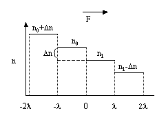
Figure B-1: Zoning Diagram for Milne's Problem

This problem has been discretized into equal sized zones with the assumption that the upper atomic population, n, is constant across a zone. Since we have focused on the right side, n can be represented by a step function with steps at each multiple of $\lambda$ as shown in Fig. B-1. In this figure, $\Delta$n is equal to n₀ - n₁. We are interested in computing F at the midpoint in terms of $\lambda$ and then relate this to the slope of the upper atomic population. Since we wish to study the effects of small optical depth per zone length, we assume $\lambda$ is much less than one. Doing so allows us to approximate the angle integrated photon density distribution by integrating the emission in each zone and differencing the flux from the right and left as

$${\frac{{1}}{{3}}} \Delta \nu \left\{\vphantom{ {\left[ {\left( {1 - e^{ - \lambda } } \right)B... ...da } - e^{ - 2\lambda } } \right)B(n_0 + \Delta n) + \cdots } \right]} }\right. \left[\vphantom{ {\left( {1 - e^{ - \lambda } } \right)B \left( {... ...{ - \lambda } - e^{ - 2\lambda } } \right)B(n_0 + \Delta n) + \cdots } }\right. \left(\vphantom{ {1 - e^{ - \lambda } } }\right. \lambda \left.\vphantom{ {1 - e^{ - \lambda } } }\right) \left(\vphantom{ {n_0 } }\right. \left.\vphantom{ {n_0 } }\right) \left(\vphantom{ {e^{ - \lambda } - e^{ - 2\lambda } } }\right. \lambda \lambda \left.\vphantom{ {e^{ - \lambda } - e^{ - 2\lambda } } }\right) \Delta \left.\vphantom{ {\left( {1 - e^{ - \lambda } } \right)B \left( {... ...{ - \lambda } - e^{ - 2\lambda } } \right)B(n_0 + \Delta n) + \cdots } }\right]$$ F =

$$\left.\vphantom{ { - \left[ {\left( {1 - e^{ - \lambda } } \right... ...da } - e^{ - 2\lambda } } \right)B(n_1 - \Delta n) + \cdots } \right]} }\right. \left[\vphantom{ {\left( {1 - e^{ - \lambda } } \right)B\left( {n... ...{ - \lambda } - e^{ - 2\lambda } } \right)B(n_1 - \Delta n) + \cdots } }\right. \left(\vphantom{ {1 - e^{ - \lambda } } }\right. \lambda \left.\vphantom{ {1 - e^{ - \lambda } } }\right) \left(\vphantom{ {n_1 } }\right. \left.\vphantom{ {n_1 } }\right) \left(\vphantom{ {e^{ - \lambda } - e^{ - 2\lambda } } }\right. \lambda \lambda \left.\vphantom{ {e^{ - \lambda } - e^{ - 2\lambda } } }\right) \Delta \left.\vphantom{ {\left( {1 - e^{ - \lambda } } \right)B\left( {n... ...{ - \lambda } - e^{ - 2\lambda } } \right)B(n_1 - \Delta n) + \cdots } }\right] \left.\vphantom{ { - \left[ {\left( {1 - e^{ - \lambda } } \right... ...a } - e^{ - 2\lambda } } \right)B(n_1 - \Delta n) + \cdots } \right]} }\right\}$$ (B-2)

The steady-state solution, B, has slightly changed from its form in equation (A-5) to its new form as

$${\frac{{{nA_{21} }}}{{{2c\left[ {K_{12} - \left( {K_{21} + K_{12} } \right)\bar n} \right]}}}}$$ (B-3)

The bracketed terms in equation (B-2) can be summed to get the following solution for F:

$${\frac{{1}}{{3}}} \Delta \nu {\frac{{{A_{21} }}}{{{2c\left[ {K_{12} - \left( {K_{21} + K_{12} } \right)\bar n} \right]}}}} \left\{\vphantom{ {n_0 - n_1 + \frac{{2e^{ - \lambda } }}{{1 - e^{ - \lambda } }} \Delta n} }\right. {\frac{{{2e^{ - \lambda } }}}{{{1 - e^{ - \lambda } }}}} \Delta \left.\vphantom{ {n_0 - n_1 + \frac{{2e^{ - \lambda } }}{{1 - e^{ - \lambda } }} \Delta n} }\right\}$$ F = (B-4)

$${\frac{{1}}{{3}}} \Delta \nu {\frac{{{A_{21} }}}{{{2c\left[ {K_{12} - \left( {K_{21} + K_{12} } \right)\bar n} \right]}}}} {\frac{{1}}{{{\tanh \left( {{\lambda \mathord{\left/ {\vphantom {\lambda 2}} \right. \kern-\nulldelimiterspace} 2}} \right)}}}}$$ =

The slope can now be approximated by using the definition of $\lambda$ from equation (B-1) along with equation (B-5) to arrive at

$${\frac{{{dn}}}{{{dx}}}} \cong {\frac{{{\Delta n}}}{{{L_{zone} }}}} {\frac{{{3\left[ {K_{12} - \left( {K_{21} + K_{12} } \right)\bar n} \right]^2 }}}{{{A_{21} \Delta \nu ^2 }}}} {\frac{{{\tanh ({\lambda \mathord{\left/ {\vphantom {\lambda 2}}... ...hord{\left/ {\vphantom {\lambda 2}} \right. \kern-\nulldelimiterspace} 2}}}}}$$ (B-5)