Milne's Problem

In our last test problem, we consider a localized source in the middle of the slab and an opacity that is independent of frequency. This approximation for the opacity, known as the grey approximation or Milne's problem [7], offers an analytical solution that can be used to check the accuracy of the numerical results.

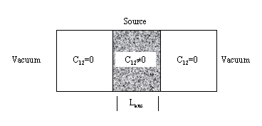
Figure 11: Milne's Problem Layout

We simulate a grey slab by defining only one energy group of width $\Delta$$\nu$. The physical configuration of this problem can be seen in Fig. 11. We define a central zone to provide a source of collisionally pumped photons of width L_exc. In this central zone, C₁₂ is to set a small value consistent with the approximations required for an analytical solution. The problem is set up with 21 equally spaced zones and the physical parameters specified in Table 3.

Table 3: Physical Parameters for Milne's Problem

The analytical solution is provided in Appendix A. We cannot easily solve for n close to the pumped region or near the edge of the slab since the boundary layers add additional complexity. However, the slope of n far from the boundaries may be obtained analytically.

The predicted slope of n versus position, equation (A-7) from the appendix, is -1.7 x 10^-4. The results of IMC and SIMC have been plotted in Fig. 12. IMC and SIMC produce slopes of -1.7 x 10^-4 and -1.3 x 10^-4, respectively. Although SIMC has a lower noise figure than IMC, as seen in this graph, it produces the wrong slope. The directional dependence of photons, $\kappa$, as defined in equation (B-1) was found experimentally to be about 1.6.

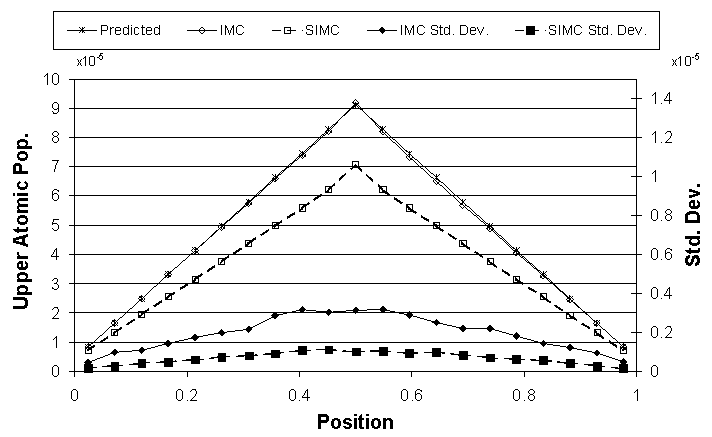
Figure 12: Results for Milne's Problem

This error for SIMC is due to the teleportation problem discussed in Sec. 2.5. When we refine the zoning by a factor of ten, which reduces the optical depth per zone, SIMC and IMC both agree with the predicted slope, -1.7 x 10^-4. Attempts to use geometric zoning schemes, with thick zones in the middle of the uniform regions on the left and right sides of this problem, suffer from the photon teleportation problems described previously.

Equation (B-5) from the appendix, displayed below, shows how teleportation error affects the predicted slopes for this problem.

$${\frac{{{dn}}}{{{dx}}}}$$ $$\cong$$ - $${\frac{{{3F\left[ {K_{12} - \left( {K_{21} + K_{12} } \right)\bar n} \right]^2 }}}{{{A_{21} \Delta \nu ^2 }}}}$$$${\frac{{{\tanh ({\lambda \mathord{\left/ {\vphantom {\lambda 2}}... ...hord{\left/ {\vphantom {\lambda 2}} \right. \kern-\nulldelimiterspace} 2}}}}}$$.

The multiplicative term, $\left[\vphantom{ {\tanh \left( {{\lambda \mathord{\left/ {\vphantom {\lambda 2}} \right. \kern-\nulldelimiterspace} 2}} \right)} }\right.$tanh$\left(\vphantom{ {{\lambda \mathord{\left/ {\vphantom {\lambda 2}} \right. \kern-\nulldelimiterspace} 2}} }\right.$$\lambda$ $\left/\vphantom{ {\vphantom {\lambda 2}} }\right.$$\vphantom$$\lambda$2-$\nulldelimiterspace$2$\left.\vphantom{ {{\lambda \mathord{\left/ {\vphantom {\lambda 2}} \right. \kern-\nulldelimiterspace} 2}} }\right)$$\left.\vphantom{ {\tanh \left( {{\lambda \mathord{\left/ {\vphantom {\lambda 2}} \right. \kern-\nulldelimiterspace} 2}} \right)} }\right]$ $\left/\vphantom{ {\vphantom {{\left[ {\tanh \left( {{\lambda \mathord{\left/ ... ...hantom {\lambda 2}} \right. \kern-\nulldelimiterspace} 2}} \right)}}} }\right.$$\vphantom$$\left[\vphantom{ {\tanh \left( {{\lambda \mathord{\left/ {\vphantom {\lambda 2}} \right. \kern-\nulldelimiterspace} 2}} \right)} }\right.$tanh$\left(\vphantom{ {{\lambda \mathord{\left/ {\vphantom {\lambda 2}} \right. \kern-\nulldelimiterspace} 2}} }\right.$$\lambda$ $\left/\vphantom{ {\vphantom {\lambda 2}} }\right.$$\vphantom$$\lambda$2-$\nulldelimiterspace$2$\left.\vphantom{ {{\lambda \mathord{\left/ {\vphantom {\lambda 2}} \right. \kern-\nulldelimiterspace} 2}} }\right)$$\left.\vphantom{ {\tanh \left( {{\lambda \mathord{\left/ {\vphantom {\lambda 2}} \right. \kern-\nulldelimiterspace} 2}} \right)} }\right]$$\left(\vphantom{ {{\lambda \mathord{\left/ {\vphantom {\lambda 2}} \right. \kern-\nulldelimiterspace} 2}} }\right.$$\lambda$ $\left/\vphantom{ {\vphantom {\lambda 2}} }\right.$$\vphantom$$\lambda$2-$\nulldelimiterspace$2$\left.\vphantom{ {{\lambda \mathord{\left/ {\vphantom {\lambda 2}} \right. \kern-\nulldelimiterspace} 2}} }\right)$-$\nulldelimiterspace$$\left(\vphantom{ {{\lambda \mathord{\left/ {\vphantom {\lambda 2}} \right. \kern-\nulldelimiterspace} 2}} }\right.$$\lambda$ $\left/\vphantom{ {\vphantom {\lambda 2}} }\right.$$\vphantom$$\lambda$2-$\nulldelimiterspace$2$\left.\vphantom{ {{\lambda \mathord{\left/ {\vphantom {\lambda 2}} \right. \kern-\nulldelimiterspace} 2}} }\right)$, modifies the slope based on the optical depth per zone, $\lambda$. As the optical depth is decreased, $\lambda$ goes to 0 and the multiplicative term asymptotically approaches 1; so it converges to the correct solution. In the other limit as the optical depth is increased, the factor goes to 0 and reduces the computed slope.

In this example problem for SIMC, $\lambda$ is 2.16 (assuming the value of $\kappa$ to be 1.6) while a tenfold increase in zoning leads to a $\lambda$ of 0.216. Since in the derivation of equation (B-5) we assumed $\lambda$ was much less than 1, we cannot use it to double check the computed slope of the example problem. However, we can see that a $\lambda$ of 0.216 yields a 0.4% error. While not derived for the collisionally pumped trap problem, it does reinforce the observation that you need finer zoning in places of large slope while zones with little to no slope do not need as much refinement.

In the IMC method, the effective scattering reduces the absorption and this must be taken into account. The resulting equation is very similar to (B-5) with a minor change. Since the absorption cross section is $\hat{f}$$\sigma$ as given in equation (10), the absorption per zone is reduced by a factor of $\hat{f}$. This results in a prediction for the slope for IMC as

$${\frac{{{dn}}}{{{dx}}}} \cong {\frac{{{3F\left[ {K_{12} - \left( {K_{21} + K_{12} } \right)\bar n} \right]^2 }}}{{{A_{21} \Delta \nu ^2 }}}} {\frac{{{\tanh \left( {{{\hat f\lambda } \mathord{\left/ {\vphan... ...antom {{\hat f\lambda } 2}} \right. \kern-\nulldelimiterspace} 2}} \right)}}}}$$ (15)

From this expression, we can see how IMC's effective scattering dampens the teleportation error. As $\hat{f}$ approaches 1 (corresponding to smaller time steps), the scattering contribution disappears and this equation approaches equation (B-5) and behaves as SIMC. As $\hat{f}$ decreases, the multiplicative term from above contributes less and less to the behavior of the slope. The limiting value of $\hat{f}$ is $\left(\vphantom{ {C_{12} + C_{21} } }\right.$C₁₂+C₂₁$\left.\vphantom{ {C_{12} + C_{21} } }\right)$/$\left(\vphantom{ {C_{12} + C_{21} + A_{21} } }\right.$C₁₂+C₂₁+A₂₁$\left.\vphantom{ {C_{12} + C_{21} + A_{21} } }\right)$ which represents the most that the teleportation error may be dampened.